![]() Follow me on twitter @bradleyboehmke
Follow me on twitter @bradleyboehmke
![]() Follow me on twitter @bradleyboehmke
Follow me on twitter @bradleyboehmke
 Classification ANNs seek to classify an observation as belonging to some discrete class as a function of the inputs. The input features (independent variables) can be categorical or numeric types, however, we require a categorical feature as the dependent variable.
In this tutorial we introduce a neural network used for numeric predictions and cover:
The following packages are required for classification ANN analysis.
library(tidyverse)
library(neuralnet)
library(GGally)
Our classification ANN will use Haberman’s Survival data set from UCI’s Machine Learning Repository. Haberman’s data set was provided by Tjen-Sien Lim email, and contains cases from a 1958 and 1970 study conducted at the University of Chicago’s Billings Hospital on the survival of 306 patients who had undergone surgery for breast cancer. We will use this data set to predict a patient’s 5-year survival as a function of their age at date of operation, year of the operation, and the number of positive axillary nodes detected.
We first download the data from UCI. When this data is imported, the Survival feature is imported as an integer, this needs to be a categorical logical value so we will modify this feature using themutate() function in the dplyr package. A value of 1 in the Survival feature indicates that the patient survived for at least 5 years after the operation, and a value of 0 indites that the patient died within 5 years.
url <- 'http://archive.ics.uci.edu/ml/machine-learning-databases//haberman/haberman.data'

Hab_Data <- read_csv(file = url,
                     col_names = c('Age', 'Operation_Year',
                                   'Number_Pos_Nodes','Survival')) %>%
  na.omit() %>%
  mutate(Survival = ifelse(Survival == 2, 0, 1),
         Survival = factor(Survival))
A brief examination of the data set…
ggpairs(Hab_Data, title = "Scatterplot Matrix of the Features of the Haberman's Survival Data Set")

shows that many more patients survived at least 5 years after the operation. Of the patients that survived (bottom-subplots of the Survival row in the Scatterplot Matrix), we see many of the patients have few numbers of positive axillary nodes detected. Examination of the Age feature shows a few of the most elderly patients died within 5 years, and of the youngest patients we see increased 5-year survivability. We forego any more detailed visual inspection in favor of learning the relationships between the features using our classification ANN.
As in the regression ANN, we must scale our features to fall on the closed $[0,1]$ interval. For classification ANNs using the neuralnet package we will not use a training and test set for model evaluation, instead we will use the Akaike Information Criterion (AIC) and Bayesian Information Criterion (BIC) for final model selection. These metrics balance the error as a function of the total number of model parameters, in the ANN case the model parameters correspond to the total number of hidden nodes.
scale01 <- function(x){
  (x - min(x)) / (max(x) - min(x))
}

Hab_Data <- Hab_Data %>%
  mutate(Age = scale01(Age),
         Operation_Year = scale01(Operation_Year),
         Number_Pos_Nodes = scale01(Number_Pos_Nodes),
         Survival = as.numeric(Survival)-1)
Classification ANNs in the neuralnet package require that the response feature, in this case Survival, be inputted as a Boolean feature. We modify the feature then run the initial classification ANN.
Hab_Data <- Hab_Data %>%
  mutate(Survival = as.integer(Survival) - 1,
         Survival = ifelse(Survival == 1, TRUE, FALSE))
We construct a 1-hidden layer ANN with 1 neuron. The neuralnet package defaults to random initial weight values, for reproducibility we set a seed and construct the network. We have added three additional arguments for the classification ANN using the neuralnet package, linear.output, err.fct, and likelihood. Setting the linear.output to FALSE and the err.fct to “ce” indicates that we are performing a classification, and forces the model to output what we may interpret as a probability of each observation belonging to Survival class 1. For classification ANN the cross-entropy error metric is more appropriate than the SSE used in regression ANNs. The likelihood argument set to TRUE indicates to neuralnet that we would like to see the AIC and BIC metrics.
set.seed(123)
Hab_NN1 <- neuralnet(Survival ~ Age + Operation_Year + Number_Pos_Nodes,
                     data = Hab_Data,
                     linear.output = FALSE,
                     err.fct = 'ce',
                     likelihood = TRUE)
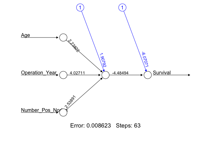
The Hab_NN1 is a list containing all parameters of the classification ANN as well as the results of the neural network on the test data set. To view a diagram of the Hab_NN1 use the plot() function.
plot(Hab_NN1, rep = 'best')
The error displayed in this plot is the cross-entropy error, which is a measure of the differences between the predicted and observed output for each of the observations in the Hab_Data data set. To view the Hab_NN1 AIC, BIC, and error metrics run the following.
Hab_NN1_Train_Error <- Hab_NN1$result.matrix[1,1]
paste("CE Error: ", round(Hab_NN1_Train_Error, 3))
## [1] "CE Error:  0.009"
Hab_NN1_AIC <- Hab_NN1$result.matrix[4,1]
paste("AIC: ", round(Hab_NN1_AIC,3))
## [1] "AIC:  12.017"
Hab_NN2_BIC <- Hab_NN1$result.matrix[5,1]
paste("BIC: ", round(Hab_NN2_BIC, 3))
## [1] "BIC:  34.359"
Classification ANNs within the neuralnet package require the use of the ce error. This forces us into using the default act.fun hyperparameter value. As a result we will only change the structure of the classification ANNs using the hidden function setting.
set.seed(123)
# 2-Hidden Layers, Layer-1 2-neurons, Layer-2, 1-neuron
Hab_NN2 <- neuralnet(Survival ~ Age + Operation_Year + Number_Pos_Nodes,
                     data = Hab_Data,
                     linear.output = FALSE,
                     err.fct = 'ce',
                     likelihood =
                       TRUE, hidden = c(2,1))

# 2-Hidden Layers, Layer-1 2-neurons, Layer-2, 2-neurons
set.seed(123)
Hab_NN3 <- Hab_NN2 <- neuralnet(Survival ~ Age + Operation_Year + Number_Pos_Nodes,
                                data = Hab_Data,
                                linear.output = FALSE,
                                err.fct = 'ce',
                                likelihood = TRUE,
                                hidden = c(2,2))

# 2-Hidden Layers, Layer-1 1-neuron, Layer-2, 2-neuron
set.seed(123)
Hab_NN4 <- Hab_NN2 <- neuralnet(Survival ~ Age + Operation_Year + Number_Pos_Nodes,
                                data = Hab_Data,
                                linear.output = FALSE,
                                err.fct = 'ce',
                                likelihood = TRUE,
                                hidden = c(1,2))

# Bar plot of results
Class_NN_ICs <- tibble('Network' = rep(c("NN1", "NN2", "NN3", "NN4"), each = 3),
                       'Metric' = rep(c('AIC', 'BIC', 'ce Error * 100'), length.out = 12),
                       'Value' = c(Hab_NN1$result.matrix[4,1], Hab_NN1$result.matrix[5,1],
                                   100*Hab_NN1$result.matrix[1,1], Hab_NN2$result.matrix[4,1],
                                   Hab_NN2$result.matrix[5,1], 100*Hab_NN2$result.matrix[1,1],
                                   Hab_NN3$result.matrix[4,1], Hab_NN3$result.matrix[5,1],
                                   100*Hab_NN3$result.matrix[1,1], Hab_NN4$result.matrix[4,1],
                                   Hab_NN4$result.matrix[5,1], 100*Hab_NN4$result.matrix[1,1]))

Class_NN_ICs %>%
  ggplot(aes(Network, Value, fill = Metric)) +
  geom_col(position = 'dodge')  +
  ggtitle("AIC, BIC, and Cross-Entropy Error of the Classification ANNs", "Note: ce Error displayed is 100 times its true value")
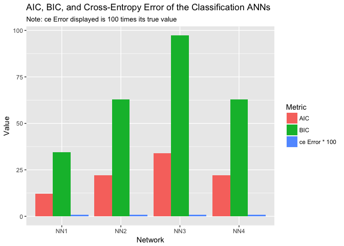
The plot indicates that as we add hidden layers and nodes within those layers, our AIC and cross-entropy error grows. The BIC appears to remain relatively constant across the designs. Here we have a case where Occam’s razor clearly applies, the ‘best’ classification ANN is the simplest.
We have briefly covered classification ANNs in this tutorial. In future tutorials we will cover more advanced applications of ANNs. Also, keep in mind that the neuralnet package used in this tutorial is only one of many tools available for ANN implementation in R. Others include:
nnetautoencodercaretRSNNSh2oBefore you move on, test your new knowledge on the exercises that follow.
Hab_Data data set.iris data set contains 4 numeric features describing 3 plant species. Think about how we would need to modify the iris data set to prepare it for a classification ANN. Hint, the data set for classification will have 7 total features.nnet has the capacity to build classification ANNs. Install and take a look at the documentation of nnet to see how it compares with neuralnet.