Real world data are often associated with dates and time; however, dealing with dates accurately can appear to be a complicated task due to the variety in formats and accounting for time-zone differences and leap years. R has a range of functions that allow you to work with dates and times. Furthermore, packages such as lubridate make it easier to work with dates and times.
In this section I will introduce you to the basics of dealing with dates. This includes:
To get current date and time information:
Sys.timezone()
## [1] "America/New_York"

Sys.Date()
## [1] "2015-09-24"

Sys.time()
## [1] "2015-09-24 15:08:57 EDT"
If using the lubridate package:
library(lubridate)

now()
## [1] "2015-09-24 15:08:57 EDT"
When date and time data are imported into R they will often default to a character string. This requires us to convert strings to dates. We may also have multiple strings that we want to merge to create a date variable.
To convert a string that is already in a date format (YYYY-MM-DD) into a date object use as.Date():
x <- c("2015-07-01", "2015-08-01", "2015-09-01")

as.Date(x)
## [1] "2015-07-01" "2015-08-01" "2015-09-01"
Note that the default date format is YYYY-MM-DD; therefore, if your string is of different format you must incorporate the format argument. There are multiple formats that dates can be in; for a complete list of formatting code options in R type ?strftime in your console.
y <- c("07/01/2015", "07/01/2015", "07/01/2015")

as.Date(y, format = "%m/%d/%Y")
## [1] "2015-07-01" "2015-07-01" "2015-07-01"
If using the lubridate package:
library(lubridate)
ymd(x)
## [1] "2015-07-01 UTC" "2015-08-01 UTC" "2015-09-01 UTC"

mdy(y)
## [1] "2015-07-01 UTC" "2015-07-01 UTC" "2015-07-01 UTC"
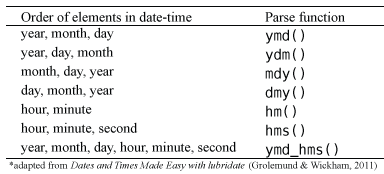
One of the many benefits of the lubridate package is that it automatically recognizes the common separators used when recording dates (“-“, “/”, “.”, and “”). As a result, you only need to focus on specifying the order of the date elements to determine the parsing function applied:

Sometimes your date data are collected in separate elements. To convert these separate data into one date object incorporate the ISOdate() function:
yr <- c("2012", "2013", "2014", "2015")
mo <- c("1", "5", "7", "2")
day <- c("02", "22", "15", "28")

# ISOdate converts to a POSIXct object
ISOdate(year = yr, month = mo, day = day)
## [1] "2012-01-02 12:00:00 GMT" "2013-05-22 12:00:00 GMT"
## [3] "2014-07-15 12:00:00 GMT" "2015-02-28 12:00:00 GMT"

# truncate the unused time data by converting with as.Date
as.Date(ISOdate(year = yr, month = mo, day = day))
## [1] "2012-01-02" "2013-05-22" "2014-07-15" "2015-02-28"
Note that ISODate() also has arguments to accept data for hours, minutes, seconds, and time-zone if you need to merge all these separate components.
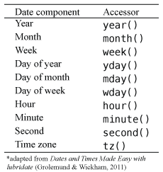
To extract and manipulate individual elements of a date I typically use the lubridate package due to its simplistic function syntax. The functions provided by lubridate to perform extraction and manipulation of dates include:

To extract an individual element of the date variable you simply use the accessor function desired. Note that the accessor variables have additional arguments that can be used to show the name of the date element in full or abbreviated form.
library(lubridate)

x <- c("2015-07-01", "2015-08-01", "2015-09-01")

year(x)
## [1] 2015 2015 2015

# default is numerical value
month(x)
## [1] 7 8 9

# show abbreviated name
month(x, label = TRUE)
## [1] Jul Aug Sep
## 12 Levels: Jan < Feb < Mar < Apr < May < Jun < Jul < Aug < Sep < ... < Dec

# show unabbreviated name
month(x, label = TRUE, abbr = FALSE)
## [1] July      August    September
## 12 Levels: January < February < March < April < May < June < ... < December


wday(x, label = TRUE, abbr = FALSE)
## [1] Wednesday Saturday  Tuesday
## 7 Levels: Sunday < Monday < Tuesday < Wednesday < Thursday < ... < Saturday
To manipulate or change the values of date elements we simply use the accessor function to extract the element of choice and then use the assignment function to assign a new value.
# convert to date format
x <- ymd(x)
x
## [1] "2015-07-01 UTC" "2015-08-01 UTC" "2015-09-01 UTC"

# change the days for the dates
mday(x)
## [1] 1 1 1

mday(x) <- c(3, 10, 22)
x
## [1] "2015-07-03 UTC" "2015-08-10 UTC" "2015-09-22 UTC"

# can also use 'update()' function
update(x, year = c(2013, 2014, 2015), month = 9)
## [1] "2013-09-03 UTC" "2014-09-10 UTC" "2015-09-22 UTC"

# can also add/subtract units
x + years(1) - days(c(2, 9, 21))
## [1] "2016-07-01 UTC" "2016-08-01 UTC" "2016-09-01 UTC"
To create a sequence of dates we can leverage the seq() function. As with numeric vectors, you have to specify at least three of the four arguments (from, to, by, and length.out).
seq(as.Date("2010-1-1"), as.Date("2015-1-1"), by = "years")
## [1] "2010-01-01" "2011-01-01" "2012-01-01" "2013-01-01" "2014-01-01"
## [6] "2015-01-01"

seq(as.Date("2015/1/1"), as.Date("2015/12/30"), by = "quarter")
## [1] "2015-01-01" "2015-04-01" "2015-07-01" "2015-10-01"

seq(as.Date('2015-09-15'), as.Date('2015-09-30'), by = "2 days")
## [1] "2015-09-15" "2015-09-17" "2015-09-19" "2015-09-21" "2015-09-23"
## [6] "2015-09-25" "2015-09-27" "2015-09-29"
Using the lubridate package is very similar. The only difference is lubridate changes the way you specify the first two arguments in the seq() function.
library(lubridate)

seq(ymd("2010-1-1"), ymd("2015-1-1"), by = "years")
## [1] "2010-01-01 UTC" "2011-01-01 UTC" "2012-01-01 UTC" "2013-01-01 UTC"
## [5] "2014-01-01 UTC" "2015-01-01 UTC"

seq(ymd("2015/1/1"), ymd("2015/12/30"), by = "quarter")
## [1] "2015-01-01 UTC" "2015-04-01 UTC" "2015-07-01 UTC" "2015-10-01 UTC"

seq(ymd('2015-09-15'), ymd('2015-09-30'), by = "2 days")
## [1] "2015-09-15 UTC" "2015-09-17 UTC" "2015-09-19 UTC" "2015-09-21 UTC"
## [5] "2015-09-23 UTC" "2015-09-25 UTC" "2015-09-27 UTC" "2015-09-29 UTC"
Creating sequences with time is very similar; however, we need to make sure our date object is POSIXct rather than just a Date object (as produced by as.Date):
seq(as.POSIXct("2015-1-1 0:00"), as.POSIXct("2015-1-1 12:00"), by = "hour")
##  [1] "2015-01-01 00:00:00 EST" "2015-01-01 01:00:00 EST"
##  [3] "2015-01-01 02:00:00 EST" "2015-01-01 03:00:00 EST"
##  [5] "2015-01-01 04:00:00 EST" "2015-01-01 05:00:00 EST"
##  [7] "2015-01-01 06:00:00 EST" "2015-01-01 07:00:00 EST"
##  [9] "2015-01-01 08:00:00 EST" "2015-01-01 09:00:00 EST"
## [11] "2015-01-01 10:00:00 EST" "2015-01-01 11:00:00 EST"
## [13] "2015-01-01 12:00:00 EST"

# with lubridate
seq(ymd_hm("2015-1-1 0:00"), ymd_hm("2015-1-1 12:00"), by = "hour")
##  [1] "2015-01-01 00:00:00 UTC" "2015-01-01 01:00:00 UTC"
##  [3] "2015-01-01 02:00:00 UTC" "2015-01-01 03:00:00 UTC"
##  [5] "2015-01-01 04:00:00 UTC" "2015-01-01 05:00:00 UTC"
##  [7] "2015-01-01 06:00:00 UTC" "2015-01-01 07:00:00 UTC"
##  [9] "2015-01-01 08:00:00 UTC" "2015-01-01 09:00:00 UTC"
## [11] "2015-01-01 10:00:00 UTC" "2015-01-01 11:00:00 UTC"
## [13] "2015-01-01 12:00:00 UTC"
Since R stores date and time objects as numbers, this allows you to perform various calculations such as logical comparisons, addition, subtraction, and working with durations.
x <- Sys.Date()
x
## [1] "2015-09-26"

y <- as.Date("2015-09-11")

x > y
## [1] TRUE

x - y
## Time difference of 15 days
The nice thing about the date/time classes is that they keep track of leap years, leap seconds, daylight savings, and time zones. Use OlsonNames() for a full list of acceptable time zone specifications.
# last leap year
x <- as.Date("2012-03-1")
y <- as.Date("2012-02-28")

x - y
## Time difference of 2 days


# example with time zones
x <- as.POSIXct("2015-09-22 01:00:00", tz = "US/Eastern")
y <- as.POSIXct("2015-09-22 01:00:00", tz = "US/Pacific")

y == x
## [1] FALSE

y - x
## Time difference of 3 hours
Similarly, the same functionality exists with the lubridate package with the only difference being the accessor function(s) used.
library(lubridate)

x <- now()
x
## [1] "2015-09-26 10:08:18 EDT"

y <- ymd("2015-09-11")

x > y
## [1] TRUE

x - y
## Time difference of 15.5891 days

y + days(4)
## [1] "2015-09-15 UTC"

x - hours(4)
## [1] "2015-09-26 06:08:18 EDT"
We can also deal with time spans by using the duration functions in lubridate. Durations simply measure the time span between start and end dates. Using base R date functions for duration calculations is tedious and often results in wrong measurements. lubridate provides simplistic syntax to calculate durations with the desired measurement (seconds, minutes, hours, etc.).
# create new duration (represented in seconds)
new_duration(60)
## [1] "60s"

# create durations for minutes, hours, years
dminutes(1)
## [1] "60s"

dhours(1)
## [1] "3600s (~1 hours)"

dyears(1)
## [1] "31536000s (~365 days)"

# add/subtract durations from date/time object
x <- ymd_hms("2015-09-22 12:00:00")

x + dhours(10)
## [1] "2015-09-22 22:00:00 UTC"

x + dhours(10) + dminutes(33) + dseconds(54)
## [1] "2015-09-22 22:33:54 UTC"
To change the time zone for a date/time we can use the with_tz() function which will also update the clock time to align with the updated time zone:
library(lubridate)

time <- now()
time
## [1] "2015-09-26 10:30:32 EDT"

with_tz(time, tzone = "MST")
## [1] "2015-09-26 07:30:32 MST"
If the time zone is incorrect or for some reason you need to change the time zone without changing the clock time you can force it with force_tz():
time
## [1] "2015-09-26 10:30:32 EDT"

force_tz(time, tzone = "MST")
## [1] "2015-09-26 10:30:32 MST"
We can also easily work with daylight savings times to eliminate impacts on date/time calculations:
# most recent daylight savings time
ds <- ymd_hms("2015-03-08 01:59:59", tz = "US/Eastern")

# if we add a duration of 1 sec we gain an extra hour
ds + dseconds(1)
## [1] "2015-03-08 03:00:00 EDT"

# add a duration of 2 hours will reflect actual daylight savings clock time
# that occured 2 hours after 01:59:59 on 2015-03-08
ds + dhours(2)
## [1] "2015-03-08 04:59:59 EDT"

# add a period of two hours will reflect clock time that normally occurs after
# 01:59:59 and is not influenced by daylight savings time.
ds + hours(2)
## [1] "2015-03-08 03:59:59 EDT"
For additional resources on learning and dealing with dates I recommend the following: