![]() Follow me on twitter @bradleyboehmke
Follow me on twitter @bradleyboehmke
![]() Follow me on twitter @bradleyboehmke
Follow me on twitter @bradleyboehmke
Artificial neural networks (ANNs) describe a specific class of machine learning algorithms designed to acquire their own knowledge by extracting useful patterns from data. ANNs are function approximators, mapping inputs to outputs, and are composed of many interconnected computational units, called neurons. Each individual neuron possesses little intrinsic approximation capability; however, when many neurons function cohesively together, their combined effects show remarkable learning performance. This tutorial provides an introduction to ANNs and discusses a few key features to consider. Future tutorials will demonstrate how to apply ANNs.
This tutorial provides a high level overview of ANNs, an analytic technique that is currently undergoing rapid development and research. To provide a robust introduction, this tutorial will cover:
ANNs are engineered computational models inspired by the brain (human & animal). While some researchers used ANNs to study animal brains, most researchers view neural networks as being inspired by, not models of, neurological systems. Figure 1 shows the basic functional unit of the brain, a biologic neuron.
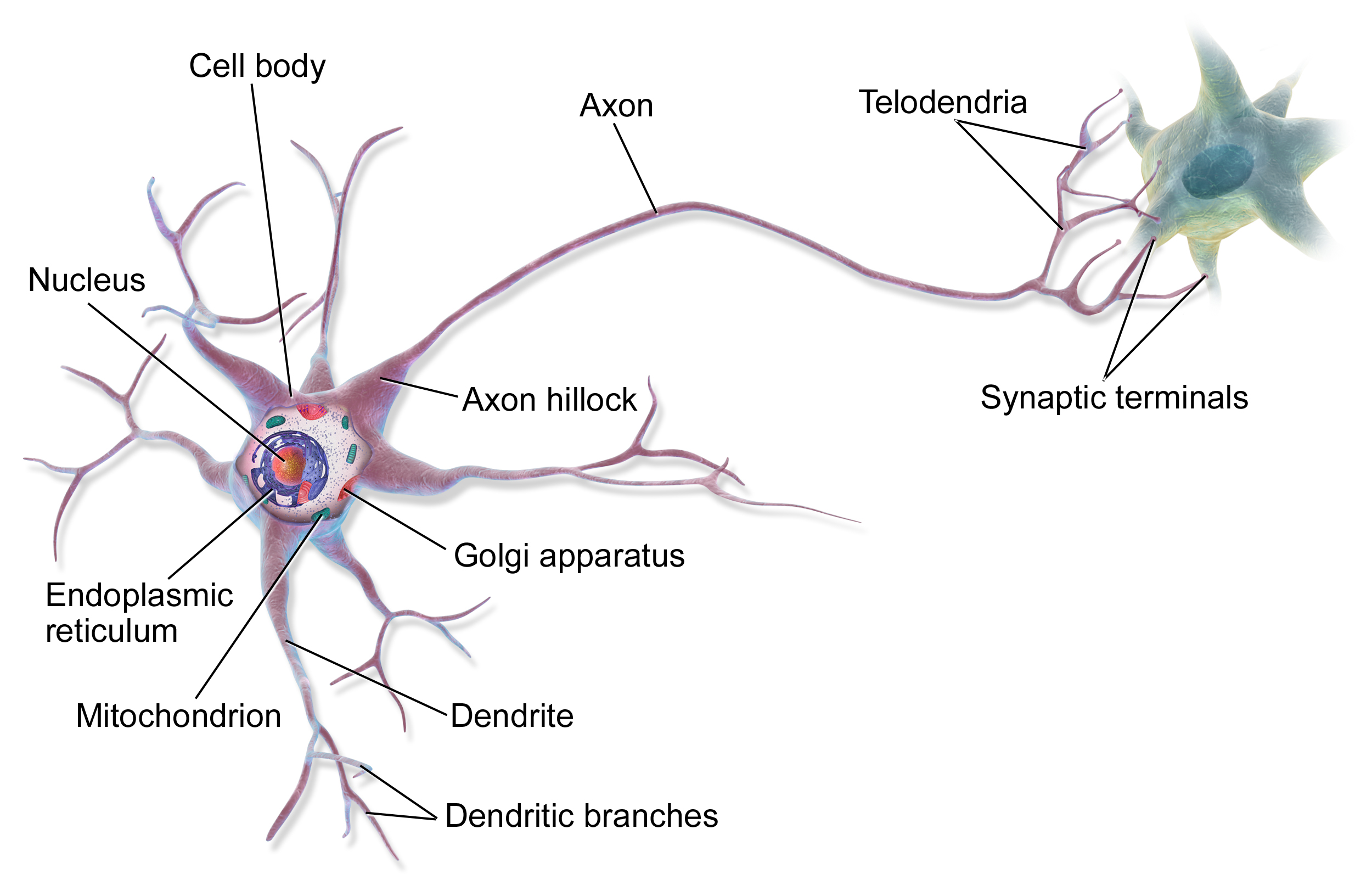
Figure 1: Biologic Neuron–Source: Bruce Blaus Wikipedia
ANN neurons are simple representations of their biologic counterparts. In the biologic neuron figure please note the Dendrite, Cell body, and the Axon with the Synaptic terminals. In biologic systems, information (in the form of neuroelectric signals) flow into the neuron through the dendrites. If a sufficient number of input signals enter the neuron through the dendrites, the cell body generates a response signal and transmits it down the axon to the synaptic terminals. The specific number of input signals required for a response signal is dependent on the individual neuron. When the generated signal reaches the synaptic terminals neurotransmitters flow out of the synaptic terminals and interact with dendrites of adjoining neurons. There are three major takeaways from the biologic neuron:
The artificial analog of the biologic neuron is shown below in figure 2. In the artificial model the inputs correspond to the dendrites, the transfer function, net input, and activation function correspond to the cell body, and the activation corresponds to the axon and synaptic terminal.

Figure 2: Artifical Neuron–Source: Chrislb Wikipedia
The inputs to the artificial neuron may correspond to raw data values, or in deeper architectures, may be outputs from preceding artificial neurons. The transfer function sums all the inputs together (cumulative inputs). If the summed input values reach a specified threshold, the activation function generates an output signal (all or nothing). The output signal then moves to a raw output or other neurons depending on specific ANN architecture. This basic artificial neuron is combined with multiple other artificial neurons to create an ANNs such as the ones shown in figure 3.


Figure 3: Examples of Multi-Neuron ANNs–Source: Click images
ANNs are often described as having an Input layer, Hidden layer, and Output layer. The input layer reads in data values from a user provided input. Within the hidden layer is where a majority of the ‘learning’ takes place, and the output layer displays the results of the ANN. In the bottom plot of the figure, each of the red input nodes correspond to an input vector . Each of the black lines with correspond to a weight, , and describe how artificial neurons are connections to one another within the ANN. The subscript identifies the source and the subscript describes to which artificial neuron the weight connects the source to. The green output nodes are the output vectors .
Examination of the figure’s top-left and top-right plots show two possible ANN configurations. In the top-left, we see a network with one hidden layer with artificial neurons, input vectors , and generates output vectors . Please note the bias inputs to each hidden node, denoted by the . The bias term is a simple constant valued 1 to each hidden node acting akin to the grand mean in a simple linear regression. Each bias term in a ANN has its own associated weight . In the top-right ANN we have a network with two hidden layers. This network adds superscript notation to the bias terms and the weights to identify to which layer each term belongs. Weights and biases with a superscript 1 act on connecting the input layer to the first layer of artificial neurons and terms with a superscript 2 connect the output of the second hidden layer to the output vectors.
The size and structure of ANNs are only limited by the imagination of the analyst.
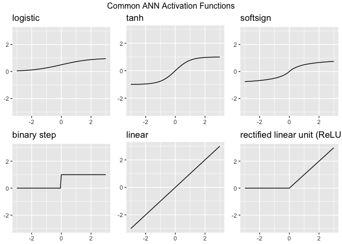
The capability of ANNs to learn approximately any function, (given sufficient training data examples) are dependent on the appropriate selection of the Activation Function(s) present in the network. Activation functions enable the ANN to learn non-linear properties present in the data. We represent the activation function here as . The input into the activation function is the weighted sum of the input features from the preceding layer. Let be the output from the jth neuron in a given layer for a network for k input vector features.
The output () can feed into the output layer of a neural network, or in deeper architectures may feed into additional hidden layers. The activation function determines if the sum of the weighted inputs plus a bias term is sufficiently large to trigger the firing of the neuron. There is not a universal best choice for the activation function, however, researchers have provided ample information regarding what activation functions work well for ANN solutions to many common problems. The choice of the activation function governs the required data scaling necessary for ANN analysis. Below we present activation functions commonly seen in may ANNs.
We have described the structure of ANNs, however, we have not touched on how these networks learn. For the purposes of this discussion we assume that we have a data set of labeled observations. Data sets in which we have some features () describing an output () fall under machine learning techniques called Supervised Learning. To begin training our notional single-layer one-neuron neural network we initially randomly assign weights. We then run the neural network with the random weights and record the outputs generated. This is called a forward pass. Output values, in our case called , are a function of the input values (), the random initial weights () and our choice of the threshold function ().
Once we have our ANN output values () we can compare them to the data set output values (). To do this we use a performance function . The choice of the performance function is a choice of the analyst, we choose to use the One-Half Square Error Cost Function otherwise known as the Sum of Squared Errors (SSE).
Now that we have our initial performance, we need a method to adjust the weights to improve the performance. For our performance function , to maximize the performance of the one-layer, one-neuron neural network, we need to minimize the difference between ANN predicted output values () and the observed data set outputs (). Recall that our neural network is simply a function, . Thus we can minimize the MSE by differentiating the performance function with respect to the weights (). Recall however, the weights in our ANN is a vector, thus we need to update each weight individually, so we require the use of the partial derivative. Additionally, we need to determine how much we want to improve. So we add a parameter , called the learning rate parameter, which is a scalar value that controls how far we move closer to the optimum weight values. The weight updates are calculated as follows:
The previous equation describes how to adjust each of the weights associated with the input features of and the bias weight . We then update the weight values as prescribed by the above equation. This process is called Back-Propagation. Once the weights are updated, we can re-run the neural network with the update weight values. This entire process can be repeated a number of times until either, a set number of iterations occur, or, we reach a pre-specified performance value (minimum error rate).
The back-propagation algorithm (described in the previous paragraphs) is the fundamental process by which an ANN learns. This brief example merely summaries high level details of the procedure. For those math-minded individuals that would like to know more, please visit Patrick H. Winston’s Neural Net Lecture. In addition to providing a good introduction to back-propagation, also provide an excellent overview to neural networks in general.
The back-propagation algorithm is the most computationally expensive component to many neural networks. Given a ANN, back-propagation requires operations for -hidden layers, and operations for the number of input weights. We often describe ANNs in terms of depth and width, where the depth refers to the number of total layers, and the width refers to the number of neurons within each layer.
Prior to moving on to ANN application we must touch on one more topic, neural network hyperparameters
ANN hyperparameters are settings used to control how a neural network performs. We have seen examples of hyperparameters previously, for example the learning rate in back-propagation and the selection of MSE as the performance metric. Hyperparameters dictate how well neural networks are able to learn the underlying functions they approximate. Poor hyperparameter selection can lead to ANNs that fail to converge, exhibit chaotic behavior, or converge too quickly at local, not global, optimums. Hyperparameters are initially selected based on historical knowledge about the data set being analyzed and/or based on the type of analysis being conducted. The optimum values of hyperparameters are dependent on the specific data sets being analyzed, therefore, in a majority of neural network analysis, hyperparameters need to be ‘tuned’ for the best performance. The No Free Lunch Theorem states that no machine learning algorithm (neural networks included) is always better at predicting new, unobserved, data points universally. When building a ANN, we are looking a building a network that performs reasonably well on a specific data set, not on all possible data sets.
The ultimate goal of an ANN is to train the network on training data, with the expectation that given new data the ANN will be able to predict their outputs with accuracy. The capability to predict new observations is called generalization. Generally, when ANNs are developed they are evaluated against one data set that has been split into a training data set and a test data set. The training data set is used to train the ANN, and the test data set is used to measure the neural networks capacity to generalize to new observations. When testing ANN hyperparameters we generally see multiple ANNs created with different hyperparameters trained on the training data set. Each of the ANNs are tested against the test data set and the ANN with the lowest test data set error is assumed to be the neural network with the best capacity to generalize to new observations.
When testing ANNs we are concerned with two types of error, under-fitting and over-fitting. An ANN exhibiting under-fitting is a neural network in which the error rate of the training data set is very high. An ANN exhibiting over-fitting has a large gap between the error rates on the training data set and the error rates on the test data set. We expect to see a slight performance decrease between the test and training data set error rates, however if this gap is large, over-fitting may be the cause. Researchers can always design a ANN with perfect performance on the training data set by increasing either the width or depth of the neural network. Adjusting these ANN hyperparameters is an adjustment of the neural networks capacity. In much the same way we can fit high-order polynomials in linear regression to perfectly match the output as a function of the regressors, ANNs can be ‘gamed’ by simply adding depth to the network. An over-capacity ANN is likely to show over-fitting when tested against the test data set. ANN’s are function approximators, and as approximators we are looking for a neural network that is no larger or complex than it needs to be for the required performance. Given two ANNs with equal test data set error performance, Occam’s razor dictates that the simplest model be selected, given no additional information.
These are some of the fundamental components of ANNs. Next you’ll learn how to apply ANNs to predict continuous and categorical outcomes.