![]() Follow me on twitter @bradleyboehmke
Follow me on twitter @bradleyboehmke
![]() Follow me on twitter @bradleyboehmke
Follow me on twitter @bradleyboehmke
 Historically, data has been available to us in the form of numeric (i.e. customer age, income, household size) and categorical features (i.e. region, department, gender). However, as organizations look for ways to collect new forms of information such as unstructured text, images, social media posts, etcetera, we need to understand how to convert this information into structured features to use in data science tasks such as customer segmentation or prediction tasks. In this tutorial, we explore a few fundamental feature engineering approaches that we can start using to convert unstructured text into structured features.
If you don’t have enough time to read through the entire post, the following hits on the key components:
Assume you work for a retailer and you currently have data on individual customer transactions for women’s clothing across. The task at the moment is to predict whether or not a customer is going to recommend a product. This task has multiple applications, for example it can
Historically, assume we only had structured features such as product name, type, class, and customer information such as age. However, recently we started collecting customer review text and this information may help improve our prediction task. But the question remains - how can we convert this unstructured text to structured features that we can use in machine learning tasks?
[1] "Absolutely wonderful - silky and sexy and comfortable"
[2] "Love this dress!  it's sooo pretty.  i happened to find it in a store, and i'm glad i did bc i never would have ordered it online bc it's petite.  i bought a petite and am 5'8\"\".  i love the length on me- hits just a little below the knee.  would definitely be a true midi on someone who is truly petite."
[3] "I had such high hopes for this dress and really wanted it to work for me. i initially ordered the petite small (my usual size) but i found this to be outrageously small. so small in fact that i could not zip it up! i reordered it in petite medium, which was just ok. overall, the top half was comfortable and fit nicely, but the bottom half had a very tight under layer and several somewhat cheap (net) over layers. imo, a major design flaw was the net over layer sewn directly into the zipper - it c"
[4] "I love, love, love this jumpsuit. it's fun, flirty, and fabulous! every time i wear it, i get nothing but great compliments!"
[5] "This shirt is very flattering to all due to the adjustable front tie. it is the perfect length to wear with leggings and it is sleeveless so it pairs well with any cardigan. love this shirt!!!"
To demonstrate various approaches in this post we’ll use Kaggle’s Women’s Clothing E-Commerce data set.
# package required
library(tidyverse)
library(tidytext)

# import data and do some initial cleaning
df <- data.table::fread("../../../Data sets/Womens Clothing E-Commerce Reviews.csv", data.table = FALSE) %>%
  rename(ID = V1) %>%
  select(-Title) %>%
  mutate(Age = as.integer(Age))

glimpse(df)
## Observations: 23,486
## Variables: 10
## $ ID                        <chr> "0", "1", "2", "3", "4", "5", "6", "...
## $ `Clothing ID`             <chr> "767", "1080", "1077", "1049", "847"...
## $ Age                       <int> 33, 34, 60, 50, 47, 49, 39, 39, 24, ...
## $ `Review Text`             <chr> "Absolutely wonderful - silky and se...
## $ Rating                    <int> 4, 5, 3, 5, 5, 2, 5, 4, 5, 5, 3, 5, ...
## $ `Recommended IND`         <int> 1, 1, 0, 1, 1, 0, 1, 1, 1, 1, 0, 1, ...
## $ `Positive Feedback Count` <int> 0, 4, 0, 0, 6, 4, 1, 4, 0, 0, 14, 2,...
## $ `Division Name`           <chr> "Initmates", "General", "General", "...
## $ `Department Name`         <chr> "Intimate", "Dresses", "Dresses", "B...
## $ `Class Name`              <chr> "Intimates", "Dresses", "Dresses", "...
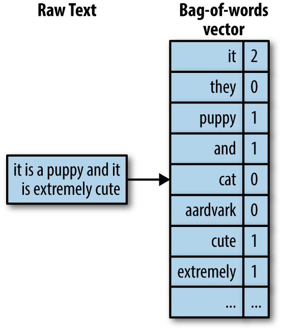
The simplest approach to convert text into structured features is using the bag of words approach. Bag of words simply breaks apart the words in the review text into individual word count statistics.
In R, we can break up our text into individual words with tidytext::unnest_tokens(). If we follow that with dplyr::count() we can sum up the unique word instances across the entire data set.
df %>%
  select(`Review Text`) %>%
  unnest_tokens(word, `Review Text`) %>%
  count(word, sort = TRUE)
## # A tibble: 14,804 x 2
##    word      n
##    <chr> <int>
##  1 the   76114
##  2 i     59237
##  3 and   49007
##  4 a     43012
##  5 it    42800
##  6 is    30640
##  7 this  25751
##  8 to    24581
##  9 in    20721
## 10 but   16554
## # ... with 14,794 more rows
To make text features more useful, informative, and to separate the wheat from the chaff we often want to perform some filtering methods.
One problem that you probably see is that our bag of words vector contains many non-informative words. Words such as “the”, “i”, “and”, “it” do not provide much context. These are considered stop words. Most of the time we want our text features to identify words that provide context (i.e. dress, love, size, flattering, etc.). Thus, we can remove the stop words from our tibble with anti_join() and the built-in stop_words data set provided by the tidytext package.
df %>%
  unnest_tokens(word, `Review Text`) %>%
  anti_join(stop_words) %>%
  count(word, sort = TRUE)
## # A tibble: 14,143 x 2
##    word           n
##    <chr>      <int>
##  1 dress      10553
##  2 love        8948
##  3 size        8768
##  4 top         7405
##  5 fit         7318
##  6 wear        6439
##  7 fabric      4790
##  8 color       4605
##  9 perfect     3772
## 10 flattering  3517
## # ... with 14,133 more rows
Now we start to see some useful information. However, if we were to look at the distribution of our word counts we see that a large portion of our words (44.6% to be exact) are only represented once.
df %>%
  unnest_tokens(word, `Review Text`) %>%
  anti_join(stop_words) %>%
  count(word) %>%
  ggplot(aes(n)) +
  geom_histogram() +
  scale_x_log10()
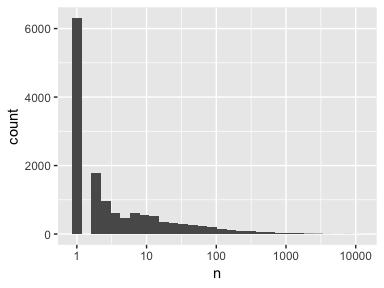
Often, low count words are obscure words, misspellings, or non-words. If we look closely at these low count words we see that many of them are truly uninformative non-words.
df %>%
  unnest_tokens(word, `Review Text`) %>%
  anti_join(stop_words) %>%
  count(word) %>%
  arrange(n)
## # A tibble: 14,143 x 2
##    word                       n
##    <chr>                  <int>
##  1 ______                     1
##  2 _________________          1
##  3 __________________         1
##  4 ______________________     1
##  5 0.02                       1
##  6 03dd                       1
##  7 04                         1
##  8 06                         1
##  9 0dd                        1
## 10 0in                        1
## # ... with 14,133 more rows
To a statistical model, a word that appears in only one or two instances is more like noise than useful information. There are several approaches to filter out these words. One approach is to use regular expressions to remove non-words. For example, the following removes any word that includes numbers, words, single letters, or words where letters are repeated 3 times (misspellings or exaggerations). However, we still have rare or infrequent words represented in our data.
df %>%
  unnest_tokens(word, `Review Text`) %>%
  anti_join(stop_words) %>%
  filter(
    !str_detect(word, pattern = "[[:digit:]]"), # removes any words with numeric digits
    !str_detect(word, pattern = "[[:punct:]]"), # removes any remaining punctuations
    !str_detect(word, pattern = "(.)\\1{2,}"),  # removes any words with 3 or more repeated letters
    !str_detect(word, pattern = "\\b(.)\\b")    # removes any remaining single letter words
    ) %>%
  count(word) %>%
  arrange(n)
## # A tibble: 12,828 x 2
##    word            n
##    <chr>       <int>
##  1 aame            1
##  2 abck            1
##  3 abdominal       1
##  4 abercrombie     1
##  5 abhor           1
##  6 abject          1
##  7 abnormal        1
##  8 abolutely       1
##  9 abruptly        1
## 10 absence         1
## # ... with 12,818 more rows
We could also filter out words based on frequency. This typically involves using a frequency cutoff value that is determined manually and shoud be re-examined when the data set changes or as models need to be updated. The following filters for all words used at least 10 or more times.
df %>%
  unnest_tokens(word, `Review Text`) %>%
  anti_join(stop_words) %>%
  filter(
    !str_detect(word, pattern = "[[:digit:]]"), # removes any words with numeric digits
    !str_detect(word, pattern = "[[:punct:]]"), # removes any remaining punctuations
    !str_detect(word, pattern = "(.)\\1{2,}"),  # removes any words with 3 or more repeated letters
    !str_detect(word, pattern = "\\b(.)\\b")    # removes any remaining single letter words
    ) %>%
  count(word) %>%
  filter(n >= 10) %>% # filter for words used 10 or more times
  arrange(n)
## # A tibble: 2,830 x 2
##    word              n
##    <chr>         <int>
##  1 accessory        10
##  2 act              10
##  3 alright          10
##  4 answer           10
##  5 anticipate       10
##  6 appropriately    10
##  7 arrives          10
##  8 backwards        10
##  9 balances         10
## 10 balls            10
## # ... with 2,820 more rows
Alternatively, you could keep all words but simply categorize low frequency words into a particular bucket. For example, the following categorizes all words that are used less than 10 times as “infrequent”.
df %>%
  unnest_tokens(word, `Review Text`) %>%
  anti_join(stop_words) %>%
  filter(
    !str_detect(word, pattern = "[[:digit:]]"), # removes any words with numeric digits
    !str_detect(word, pattern = "[[:punct:]]"), # removes any remaining punctuations
    !str_detect(word, pattern = "(.)\\1{2,}"),  # removes any words with 3 or more repeated letters
    !str_detect(word, pattern = "\\b(.)\\b")    # removes any remaining single letter words
    ) %>%
  count(word) %>%
  mutate(word = if_else(n < 10, "infrequent", word)) %>% # categorize infrequent words
  group_by(word) %>%
  summarize(n = sum(n)) %>%
  arrange(desc(n))
## # A tibble: 2,831 x 2
##    word           n
##    <chr>      <int>
##  1 infrequent 22847
##  2 dress      10553
##  3 love        8948
##  4 size        8768
##  5 top         7405
##  6 fit         7318
##  7 wear        6439
##  8 fabric      4790
##  9 color       4605
## 10 perfect     3772
## # ... with 2,821 more rows
Even after we’ve filtered for only informative words, sometimes we have multiple words that represent the same meaning (are mapped to the same word) but have slightly different spelling due to sentence context. For example, “love”, “loving”, “lovingly”, “loved”, and “lovely” could all be used by customers to illustrate they love something. Word stemming is a task that chops each word down to its basic linguistic word stem form. We can stem words using the corpus::text_tokens() function.
text <- c("love", "loving", "lovingly", "loved", "lovely")
corpus::text_tokens(text, stemmer = "en") %>% unlist()
## [1] "love" "love" "love" "love" "love"
We can easily add this into our filtering process adding a mutate() call after filter().
Note: There is on-going debate about the benefits of stemming. Consequently, its usually useful to assess how non-stemmed features perform versus stemmed features in your predictive modeling.
df %>%
  unnest_tokens(word, `Review Text`) %>%
  anti_join(stop_words) %>%
  filter(
    !str_detect(word, pattern = "[[:digit:]]"),
    !str_detect(word, pattern = "[[:punct:]]"),
    !str_detect(word, pattern = "(.)\\1{2,}"),
    !str_detect(word, pattern = "\\b(.)\\b")
    ) %>%
  mutate(word = corpus::text_tokens(word, stemmer = "en") %>% unlist()) %>% # add stemming process
  count(word) %>%
  group_by(word) %>%
  summarize(n = sum(n)) %>%
  arrange(desc(n))
## # A tibble: 8,789 x 2
##    word        n
##    <chr>   <int>
##  1 dress   12173
##  2 fit     11504
##  3 love    11392
##  4 size    10716
##  5 top      8360
##  6 wear     8075
##  7 color    7299
##  8 perfect  5282
##  9 fabric   4885
## 10 nice     3819
## # ... with 8,779 more rows
Ok, so assume we’ve decided to simply filter out infrequent and non-informative words. The next question is how do we add these as features to our original data set? First, we create a vector of all words that we want to keep (this is based on filtering out stop words, non-informative words, and only words used at least 10 times or more). Then we can use that word list to filter for only those words and then we summarize the count for each word at the customer ID level. What results is a very wide and sparse feature set as many of the customers will have a majority of 0’s across these newly created 2,830 features.
# create a vector of all words to keep
word_list <- df %>%
  unnest_tokens(word, `Review Text`) %>%
  anti_join(stop_words) %>%
  filter(
    !str_detect(word, pattern = "[[:digit:]]"), # removes any words with numeric digits
    !str_detect(word, pattern = "[[:punct:]]"), # removes any remaining punctuations
    !str_detect(word, pattern = "(.)\\1{2,}"),  # removes any words with 3 or more repeated letters
    !str_detect(word, pattern = "\\b(.)\\b")    # removes any remaining single letter words
    ) %>%
  count(word) %>%
  filter(n >= 10) %>% # filter for words used 10 or more times
  pull(word)

# create new features
bow_features <- df %>%
  unnest_tokens(word, `Review Text`) %>%
  anti_join(stop_words) %>%
  filter(word %in% word_list) %>%     # filter for only words in the wordlist
  count(ID, word) %>%                 # count word useage by customer ID
  spread(word, n) %>%                 # convert to wide format
  map_df(replace_na, 0)               # replace NAs with 0

bow_features
## # A tibble: 22,640 x 2,831
##    ID    ability absolute absolutely   abt accent accents accentuate
##    <chr>   <dbl>    <dbl>      <dbl> <dbl>  <dbl>   <dbl>      <dbl>
##  1 0           0        0          1     0      0       0          0
##  2 1           0        0          0     0      0       0          0
##  3 10          0        0          0     0      0       0          0
##  4 100         0        0          0     0      0       0          0
##  5 1000        0        0          0     0      0       0          0
##  6 10000       0        0          0     0      0       0          0
##  7 10001       0        0          0     0      0       0          0
##  8 10002       0        0          0     0      0       0          0
##  9 10003       0        0          0     0      0       0          0
## 10 10004       0        0          0     0      0       0          0
## # ... with 22,630 more rows, and 2,823 more variables: accentuated <dbl>,
## #   accentuates <dbl>, acceptable <dbl>, accessories <dbl>,
## #   accessorize <dbl>, accessory <dbl>, accidentally <dbl>,
## #   accommodate <dbl>, accurate <dbl>, accurately <dbl>, achieve <dbl>,
## #   acrylic <dbl>, act <dbl>, active <dbl>, actual <dbl>, add <dbl>,
## #   added <dbl>, adding <dbl>, addition <dbl>, additional <dbl>,
## #   additionally <dbl>, adds <dbl>, adequate <dbl>, adjust <dbl>,
## #   adjustable <dbl>, adjusted <dbl>, adjusting <dbl>, admit <dbl>,
## #   adn <dbl>, adorable <dbl>, adore <dbl>, adored <dbl>, advantage <dbl>,
## #   advertised <dbl>, advice <dbl>, aesthetic <dbl>, affordable <dbl>,
## #   afraid <dbl>, afternoon <dbl>, ag <dbl>, age <dbl>, ages <dbl>,
## #   ago <dbl>, agree <dbl>, agreed <dbl>, ahead <dbl>, air <dbl>,
## #   airy <dbl>, aka <dbl>, alas <dbl>, albeit <dbl>, allowing <dbl>,
## #   alot <dbl>, alright <dbl>, alter <dbl>, alteration <dbl>,
## #   alterations <dbl>, altered <dbl>, altering <dbl>, alternative <dbl>,
## #   amazed <dbl>, amazing <dbl>, amazingly <dbl>, amount <dbl>, amp <dbl>,
## #   ample <dbl>, angel <dbl>, angle <dbl>, angles <dbl>, animal <dbl>,
## #   ankle <dbl>, ankles <dbl>, annoying <dbl>, answer <dbl>, antho <dbl>,
## #   anticipate <dbl>, anticipated <dbl>, antro <dbl>, anymore <dbl>,
## #   anytime <dbl>, apparent <dbl>, apparently <dbl>, appeal <dbl>,
## #   appealing <dbl>, appearance <dbl>, appeared <dbl>, appears <dbl>,
## #   apple <dbl>, appliquã <dbl>, appreciated <dbl>, appropriately <dbl>,
## #   approx <dbl>, aqua <dbl>, arm <dbl>, armhole <dbl>, armholes <dbl>,
## #   armpit <dbl>, armpits <dbl>, arms <dbl>, army <dbl>, …
Now we can add these features by joining this new feature set to the original feature set using the ID variable as the key.
# join original data and new feature set together
df_bow <- df %>%
  inner_join(bow_features, by = "ID") %>%   # join data sets
  select(-`Review Text`)                    # remove original review text

# dimension of our new data set
dim(df_bow)
## [1] 22640  2839

as_tibble(df_bow)
## # A tibble: 22,640 x 2,839
##    ID    `Clothing ID`   Age Rating `Recommended IN… `Positive Feedb…
##    <chr> <chr>         <int>  <int>            <int>            <int>
##  1 0     767              33      4                1                0
##  2 1     1080             34      5                1                4
##  3 2     1077             60      3                0                0
##  4 3     1049             50      5                1                0
##  5 4     847              47      5                1                6
##  6 5     1080             49      2                0                4
##  7 6     858              39      5                1                1
##  8 7     858              39      4                1                4
##  9 8     1077             24      5                1                0
## 10 9     1077             34      5                1                0
## # ... with 22,630 more rows, and 2,833 more variables: `Division
## #   Name` <chr>, `Department Name` <chr>, `Class Name` <chr>,
## #   ability <dbl>, absolute <dbl>, absolutely <dbl>, abt <dbl>,
## #   accent <dbl>, accents <dbl>, accentuate <dbl>, accentuated <dbl>,
## #   accentuates <dbl>, acceptable <dbl>, accessories <dbl>,
## #   accessorize <dbl>, accessory <dbl>, accidentally <dbl>,
## #   accommodate <dbl>, accurate <dbl>, accurately <dbl>, achieve <dbl>,
## #   acrylic <dbl>, act <dbl>, active <dbl>, actual <dbl>, add <dbl>,
## #   added <dbl>, adding <dbl>, addition <dbl>, additional <dbl>,
## #   additionally <dbl>, adds <dbl>, adequate <dbl>, adjust <dbl>,
## #   adjustable <dbl>, adjusted <dbl>, adjusting <dbl>, admit <dbl>,
## #   adn <dbl>, adorable <dbl>, adore <dbl>, adored <dbl>, advantage <dbl>,
## #   advertised <dbl>, advice <dbl>, aesthetic <dbl>, affordable <dbl>,
## #   afraid <dbl>, afternoon <dbl>, ag <dbl>, age <dbl>, ages <dbl>,
## #   ago <dbl>, agree <dbl>, agreed <dbl>, ahead <dbl>, air <dbl>,
## #   airy <dbl>, aka <dbl>, alas <dbl>, albeit <dbl>, allowing <dbl>,
## #   alot <dbl>, alright <dbl>, alter <dbl>, alteration <dbl>,
## #   alterations <dbl>, altered <dbl>, altering <dbl>, alternative <dbl>,
## #   amazed <dbl>, amazing <dbl>, amazingly <dbl>, amount <dbl>, amp <dbl>,
## #   ample <dbl>, angel <dbl>, angle <dbl>, angles <dbl>, animal <dbl>,
## #   ankle <dbl>, ankles <dbl>, annoying <dbl>, answer <dbl>, antho <dbl>,
## #   anticipate <dbl>, anticipated <dbl>, antro <dbl>, anymore <dbl>,
## #   anytime <dbl>, apparent <dbl>, apparently <dbl>, appeal <dbl>,
## #   appealing <dbl>, appearance <dbl>, appeared <dbl>, appears <dbl>,
## #   apple <dbl>, appliquã <dbl>, appreciated <dbl>, …
Bag of n-grams is a natural extension of bag of words. An n-gram is simply any sequence of n tokens (words). Consequently, given the following review text - “Absolutely wonderful - silky and sexy and comfortable”, we could break this up into:
Bag of n-grams can be more informative than bag of words because they capture more context around each word (i.e. “love this dress” is more informative than just “dress”). However, this comes at a cost as bag of n-grams can produce a much larger and sparser feature set than bag of words (filtering methods help to minimize this). Typically, 3-grams is about as high as we want to go as using higher n-grams beyond that rarely increases performance because of sparsity.
Creating n-grams follows a similar process as with bag of words, however, we just need to add some arguments to the unnest_tokens() function:
# create bigrams
df %>%
  unnest_tokens(bigram, `Review Text`, token = "ngrams", n = 2) %>%
  head()
##   ID Clothing ID Age Rating Recommended IND Positive Feedback Count
## 1  0         767  33      4               1                       0
## 2  0         767  33      4               1                       0
## 3  0         767  33      4               1                       0
## 4  0         767  33      4               1                       0
## 5  0         767  33      4               1                       0
## 6  0         767  33      4               1                       0
##   Division Name Department Name Class Name               bigram
## 1     Initmates        Intimate  Intimates absolutely wonderful
## 2     Initmates        Intimate  Intimates      wonderful silky
## 3     Initmates        Intimate  Intimates            silky and
## 4     Initmates        Intimate  Intimates             and sexy
## 5     Initmates        Intimate  Intimates             sexy and
## 6     Initmates        Intimate  Intimates      and comfortable
To create our 2-gram feature set we can follow a very similar process as we did with the bag of words. First, we create our list of bi-grams to keep. We have to take a few extra steps in the filtering process since we are working with multiple words. Essentially, we break apart our bi-gram, filter out any part of the bi-gram that contains a stop word or other non-informative word, re-unite the bi-gram and only keep those bigrams used 10 or more times.
We can then use this list to filter our bi-grams, count the bi-gram usage by customer, and create our wide/sparse bi-gram feature set. Now we have the bi-gram feature set that we could join to our original feature set as before.
# create a vector of all bi-grams to keep
ngram_list <- df %>%
  unnest_tokens(bigram, `Review Text`, token = "ngrams", n = 2) %>%
  separate(bigram, c("word1", "word2"), sep = " ") %>%
  filter(
    !word1 %in% stop_words$word,                 # remove stopwords from both words in bi-gram
    !word2 %in% stop_words$word,
    !str_detect(word1, pattern = "[[:digit:]]"), # removes any words with numeric digits
    !str_detect(word2, pattern = "[[:digit:]]"),
    !str_detect(word1, pattern = "[[:punct:]]"), # removes any remaining punctuations
    !str_detect(word2, pattern = "[[:punct:]]"),
    !str_detect(word1, pattern = "(.)\\1{2,}"),  # removes any words with 3 or more repeated letters
    !str_detect(word2, pattern = "(.)\\1{2,}"),
    !str_detect(word1, pattern = "\\b(.)\\b"),   # removes any remaining single letter words
    !str_detect(word1, pattern = "\\b(.)\\b")
    ) %>%
  unite("bigram", c(word1, word2), sep = " ") %>%
  count(bigram) %>%
  filter(n >= 10) %>% # filter for bi-grams used 10 or more times
  pull(bigram)

# sneak peek at our bi-gram list
head(ngram_list)
## [1] "absolutely adorable"  "absolutely adore"     "absolutely beautiful"
## [4] "absolutely fell"      "absolutely gorgeous"  "absolutely love"

# create new bi-gram features
ngram_features <- df %>%
  unnest_tokens(bigram, `Review Text`, token = "ngrams", n = 2) %>%
  filter(bigram %in% ngram_list) %>%    # filter for only bi-grams in the ngram_list
  count(ID, bigram) %>%                 # count bi-gram useage by customer ID
  spread(bigram, n) %>%                 # convert to wide format
  map_df(replace_na, 0)                 # replace NAs with 0

ngram_features
## # A tibble: 17,286 x 1,354
##    ID    `absolutely ado… `absolutely ado… `absolutely bea…
##    <chr>            <dbl>            <dbl>            <dbl>
##  1 10                   0                0                0
##  2 100                  0                0                0
##  3 1000                 0                0                0
##  4 10000                0                0                0
##  5 10001                0                0                0
##  6 10002                0                0                0
##  7 10005                0                0                0
##  8 10006                0                0                0
##  9 10007                0                0                0
## 10 10008                0                0                0
## # ... with 17,276 more rows, and 1,350 more variables: `absolutely
## #   fell` <dbl>, `absolutely gorgeous` <dbl>, `absolutely love` <dbl>,
## #   `absolutely loved` <dbl>, `absolutely lovely` <dbl>, `absolutely
## #   perfect` <dbl>, `absolutely stunning` <dbl>, `add bulk` <dbl>, `added
## #   bonus` <dbl>, `adjustable straps` <dbl>, `adorable dress` <dbl>,
## #   `adorable top` <dbl>, `ag jeans` <dbl>, `ag stevie` <dbl>, `air
## #   dried` <dbl>, `air dry` <dbl>, `air drying` <dbl>, `amazing
## #   dress` <dbl>, `amazingly soft` <dbl>, `amp amp` <dbl>, `ankle
## #   bone` <dbl>, `ankle boots` <dbl>, `ankle jeans` <dbl>, `ankle
## #   length` <dbl>, `ankle pants` <dbl>, `appears online` <dbl>, `arm
## #   hole` <dbl>, `arm holes` <dbl>, `arm length` <dbl>, `arm
## #   movement` <dbl>, `arm openings` <dbl>, `arms fit` <dbl>, `army
## #   green` <dbl>, `asymmetrical hem` <dbl>, `athletic build` <dbl>,
## #   `athletic frame` <dbl>, `average height` <dbl>, `baby belly` <dbl>,
## #   `baby bump` <dbl>, `baby doll` <dbl>, `baby shower` <dbl>, `baby
## #   weight` <dbl>, `ballet flats` <dbl>, `barely fit` <dbl>, `basic
## #   tee` <dbl>, `basic top` <dbl>, `bathing suit` <dbl>, `bathing
## #   suits` <dbl>, `beach cover` <dbl>, `beautiful blouse` <dbl>,
## #   `beautiful blue` <dbl>, `beautiful coat` <dbl>, `beautiful
## #   color` <dbl>, `beautiful colors` <dbl>, `beautiful design` <dbl>,
## #   `beautiful detail` <dbl>, `beautiful details` <dbl>, `beautiful
## #   drape` <dbl>, `beautiful dress` <dbl>, `beautiful embroidery` <dbl>,
## #   `beautiful fabric` <dbl>, `beautiful flattering` <dbl>, `beautiful
## #   lace` <dbl>, `beautiful material` <dbl>, `beautiful pattern` <dbl>,
## #   `beautiful piece` <dbl>, `beautiful print` <dbl>, `beautiful
## #   quality` <dbl>, `beautiful rich` <dbl>, `beautiful shade` <dbl>,
## #   `beautiful shirt` <dbl>, `beautiful skirt` <dbl>, `beautiful
## #   soft` <dbl>, `beautiful sweater` <dbl>, `beautiful top` <dbl>,
## #   `beautifully designed` <dbl>, `beige color` <dbl>, `bell shape` <dbl>,
## #   `bell shaped` <dbl>, `bell sleeve` <dbl>, `bell sleeves` <dbl>, `belly
## #   button` <dbl>, `bigger size` <dbl>, `birthday discount` <dbl>,
## #   `birthday gift` <dbl>, `bit baggy` <dbl>, `bit boxy` <dbl>, `bit
## #   darker` <dbl>, `bit disappointed` <dbl>, `bit heavy` <dbl>, `bit
## #   itchy` <dbl>, `bit larger` <dbl>, `bit loose` <dbl>, `bit
## #   looser` <dbl>, `bit low` <dbl>, `bit lower` <dbl>, `bit odd` <dbl>,
## #   `bit oversized` <dbl>, `bit pricey` <dbl>, `bit roomy` <dbl>, …
So far we have been using raw counts for our text features and primarily did filtering based on frequency. Alternatively, we can use more robust statistical measures to determine if the observed words in an n-gram have a higher likelihood of being used together versus independently of one another. This can help detect unique phrases that are more likely to be used together versus not (i.e. “witch hunt” is more probable than the use of “witch” or “hunt” independently or with other words).
The log likelihood ratio test for bi-grams tests how much more likely one hypothesis is than than another. More specifically, we are testing how more likely word 2 occurs when word 1 precedes it in a bi-gram. So basically is the hypothesis that the probability of word 2 occurring when word 1 precedes it is equal to the probability of word 2 occurring when word 1 does not precede it. Whereas is the hypothesis that these probabilities are not equal.
To test this we use Equation 3 which takes the log of the likelihood over the likelihood of :
The steps to compute the likelihood ratio test include:
To perform the likelihood ratio test in R, first we’ll break up our review text into bi-grams and keep the actual bi-gram separated as two words.
# create bi-grams and clean them up.
bigrams <- df %>%
  select(`Review Text`) %>%
  unnest_tokens(bigram, `Review Text`, token = "ngrams", n = 2) %>%
  filter(bigram %in% ngram_list) %>%
  separate(bigram, c("word1", "word2"), sep = " ")

# sneak peak
head(bigrams)
##         word1  word2
## 1 comfortable   love
## 2       usual   size
## 3      petite medium
## 4         top   half
## 5         fit nicely
## 6      bottom   half
Next, we get our word and bi-gram counts. We also need the original number of total bi-grams (N) - not just unique bi-grams. Lastly, we use this information to compute a few probabilities and the log likelihood values (LL).
Note: I’m skipping over a lot of details here so if you want to dig deeper into what is going on check out Stanford’s book on Foundation’s of Statistical Natural Language Processing.
# compute counts for word 1 & 2 independently
count_w1 <- bigrams %>%
  count(word1)

count_w2 <- bigrams %>%
  count(word2)

# compute counts for bi-grams
count_w12 <- bigrams %>%
  count(word1, word2)

# get the original number of all bi-grams
N <- nrow(bigrams)

# join this information and compute log-likelihood
LL_test <- count_w12 %>%
  left_join(count_w1, by = "word1") %>%
  left_join(count_w2, by = "word2") %>%
  rename(c_w1 = n.y, c_w2 = n, c_w12 = n.x) %>%
  mutate(
    p = c_w2 / N,
    p1 = c_w12 / c_w1,
    p2 = (c_w2 - c_w12) / (N - c_w1),
    LL = log((pbinom(c_w12, c_w1, p) * pbinom(c_w2 - c_w12, N - c_w1, p)) / (pbinom(c_w12, c_w1, p1) * pbinom(c_w2 - c_w12, N - c_w1, p)))
  )
head(LL_test)
## # A tibble: 6 x 9
##   word1      word2     c_w12  c_w1  c_w2        p     p1       p2    LL
##   <chr>      <chr>     <int> <int> <int>    <dbl>  <dbl>    <dbl> <dbl>
## 1 absolutely adorable     22   614    32 0.000817 0.0358 0.000259 0.586
## 2 absolutely adore        26   614    26 0.000663 0.0423 0        0.594
## 3 absolutely beautiful   100   614   125 0.00319  0.163  0.000648 0.641
## 4 absolutely fell         15   614    27 0.000689 0.0244 0.000311 0.565
## 5 absolutely gorgeous     63   614    63 0.00161  0.103  0        0.628
## 6 absolutely love        301   614   932 0.0238   0.490  0.0164   0.661
The nice thing about these log likelihood values, if we multiply them by -2 then they align to the distribution. Consequently, we can now use a p-value of interest to determine a cut-off. The following takes all bi-grams where the log likelihood p-value is less than 0.05. This provides us with a list of 258 “unique” bi-grams where word 2 is strongly tied to the word that precedes it. As before we could proceed to create our new text features based on these bi-grams and join them to our original feature set.
#
unique_bigrams <- LL_test %>%
  mutate(
    Chi_value = -2 * LL,
    pvalue = pchisq(LL, df = 1)
  ) %>%
  filter(pvalue < 0.05) %>%
  select(word1, word2) %>%
  unite(bigram, word1, word2, sep = " ")

head(unique_bigrams)
## # A tibble: 6 x 1
##   bigram
##   <chr>
## 1 add bulk
## 2 added bonus
## 3 adjustable straps
## 4 amazing dress
## 5 amazingly soft
## 6 amp amp
So far we have been creating features from all words regardless of their semantic purpose. There may be times where we want to use words that have specific purposes such as nouns, verbs, and adjectives. To get this information from text we need to perform parts-of-speech (POS) tagging. There are a few different packages that can provide POS tagging. One is RDRPOSTagger. Note: RDRPOSTagger is not available on CRAN but can be downloaded from https://github.com/bnosac/RDRPOSTagger. This is not recommended on the servers but there are alternative packages on CRAN that can perform the same task (i.e. qdap). This is primarily for illustrative purposes.
words <- c("the", "quick", "brown", "fox", "jumps", "over", "the", "lazy", "dog")

# define the language and the type of tagging
tagger <- RDRPOSTagger::rdr_model(language = "English", annotation = "UniversalPOS")

# perform parts-of-speech tagging
RDRPOSTagger::rdr_pos(tagger, x = words)
##   doc_id token_id token  pos
## 1     d1        1   the  DET
## 2     d2        1 quick  ADJ
## 3     d3        1 brown  ADJ
## 4     d4        1   fox NOUN
## 5     d5        1 jumps VERB
## 6     d6        1  over  ADP
## 7     d7        1   the  DET
## 8     d8        1  lazy  ADJ
## 9     d9        1   dog NOUN
To tag the POS for our review text, first I filter down to the informative words that I identified earlier in this post. I then perform the POS tagging within mutate() and extract just the pos output that we saw in the above data frame. We now have every informative word tagged with its POS and we can use this information in several ways:
Whichever approach you perform, the process of developing the new feature set and joining to the original features follows very similar steps as we performed earlier.
# step 1: get informative words
bow <- df %>%
  select(`Review Text`) %>%
  unnest_tokens(word, `Review Text`) %>%
  anti_join(stop_words) %>%
  filter(word %in% word_list)

# step 2: POS tagging
bow_pos <- mutate(bow, pos = RDRPOSTagger::rdr_pos(tagger, x = word)$pos)

head(bow_pos, 20)
##                 word   pos
## 1               love  VERB
## 2              dress  NOUN
## 3              store  NOUN
## 4               glad   ADJ
## 5                 bc  NOUN
## 6                 bc  NOUN
## 7             bought  VERB
## 8               love  VERB
## 9             length  NOUN
## 10              knee  NOUN
## 11              true   ADJ
## 12              midi PROPN
## 13             dress  NOUN
## 14             usual   ADJ
## 15              size  NOUN
## 16             found  VERB
## 17               zip  NOUN
## 18            medium  NOUN
## 19               top  NOUN
## 20              half  NOUN
This post was designed to introduce you to different ways that we can extract features from unstructured text. This is not all inclusive and, in fact, future posts will likely discuss additional methods for extracting text features (i.e. tf-idf, word2vec). What is important to realize is there are many ways we can extract text features to include in our data sets for modeling purposes (both unsupervised and supervised).
To learn more about working with unstructured text check out the following resources: