↩

Imprecise Regression

Imprecise regression is a generalization of linear regression that gives us stronger tools for modeling uncertainty. In a typical linear regression setting, we consider the input data to be precise observations: single points. In imprecise regression, we generalize the notion of observations to intervals rather than points. This allows us to more accurately represent scenarios with measurement error or other sources of uncertainty that make our input data “fuzzy”. In many regression applications, the error introduced by treating the observations as precise numbers is insignificant. However, when there is deep uncertainty or high sensitivity to changes in the model, imprecise regression is appropriate.

This tutorial is based on the imprecise regression work in Cattaneo and Wiencierz (2012).

tl;dr

Imprecise regression, and imprecise probability more generally, is still a relatively young field. Imprecise regression can refer to several different modeling approaches, but this tutorial will focus on likelihood-based imprecise regression (LIR) for interval data.

Replication requirements: What you’ll need to reproduce the analysis.
Data preparation: Creating the necessary data structure.
Imprecise probability: Understanding imprecise probability theory.
Likelihood-based imprecise regression: A simple regression illustration.
Other approaches: Alternative approaches to imprecise regression.
Exercises: Apply what you learned.

Replication requirements

The linLIR package has significant compatibility issues. To use this package, it’s important to restart R without loading any other packages.

For this tutorial, we’ll use a toy data set from linLIR called toy.smps. This is a sample data set with two undefined variables that each have a lower and upper value recorded for every observation. There are 17 total observations in the dataset. We’ll consider a more concrete dataset in the exercises, but for now the toy dataset will help highlight some unusual aspects of imprecise regression.

# Packages
library(linLIR) 

# Load data
data("toy.smps")
data_df = data.frame(toy.smps)

data_df
##      V1   V2   V3  V4
## 1  -1.9 -1.4  2.4 2.9
## 2  -1.8 -1.6  2.7 2.8
## 3  -1.5 -1.4  2.2 2.3
## 4  -1.3 -1.1  1.9 2.1
## 5  -0.9 -0.9  1.7 2.2
## 6  -0.7 -0.5  1.7 2.1
## 7  -0.4  0.0  1.1 1.4
## 8  -0.2  0.5  1.3 1.5
## 9   0.2  0.3  1.0 1.1
## 10  0.4  0.7  0.8 1.1
## 11  1.0  1.0  1.0 1.0
## 12  1.0  1.6  0.6 0.7
## 13  1.2  1.3 -Inf 0.9
## 14  1.6  Inf  0.4 0.4
## 15  1.8  1.9  0.1 0.2
## 16  5.2  5.3  5.8 6.0
## 17  5.5  6.0  4.7 5.0

Data preparation

To use the linLIR package, we need to convert our data to a specialized data structure class idf, interval data frame. You may have noticed that there are two values that are recorded as infinite. In traditional regression, we’d have to consider using missing data or imputation methods, but since we’ll be using imprecise regression we can keep the infinite values as they are. We’ll label the independent variable “x” and the dependent variable “y”, with the lower and upper bounds of the intervals denoted “x.l”,”x.u” and “y.l”,”y.u” respectively.

data_idf <- idf.create(toy.smps, var.labels = c("x", "y"))
summary(data_idf)
## 
## Summary of interval data frame
## 
## 17 observations
## 2 interval-valued variables 
## 
## Variable x : 
## 
##       x.l               x.u      
##  Min.   :-1.9000   Min.   :-1.6  
##  1st Qu.:-0.9000   1st Qu.:-0.9  
##  Median : 0.2000   Median : 0.5  
##  Mean   : 0.5412   Mean   : Inf  
##  3rd Qu.: 1.2000   3rd Qu.: 1.6  
##  Max.   : 5.5000   Max.   : Inf  
## 
## Variable y : 
## 
##       y.l            y.u       
##  Min.   :-Inf   Min.   :0.200  
##  1st Qu.: 0.8   1st Qu.:1.000  
##  Median : 1.3   Median :1.500  
##  Mean   :-Inf   Mean   :1.982  
##  3rd Qu.: 2.2   3rd Qu.:2.300  
##  Max.   : 5.8   Max.   :6.000

Imprecise probability

Imprecise probability can be considered a generalization of traditional probability theory, motivated in part by the shortcomings of precise probabilities in expressing ambiguity or deep uncertainty. At the most general level, the theory of sets of desirable gambles serves as a foundation for the imprecise probability framework. Precise probability theory can then be derived as a special case from this theory. Related topics such as p-boxes, belief functions, possibility theory, fuzzy statistics, and robust Bayesian approaches can also be interpreted as special cases of the theory of sets of desirable gambles. One of the most applicable special cases is interval probabilities, which replace single-point probabilities with intervals of probabilities. In recent years, practical results for statistical inference and modeling in an imprecise framework have also been published.

In imprecise probability, we make a careful distinction between two broad categories of uncertainty: aleatoric and epistemic. Aleatoric uncertainty, also called irreducible uncertainty, is uncertainty due to variation. Epistemic uncertainty, also called reducible uncertainty, is uncertainty due to incomplete knowledge. Consider the simple example of flipping a coin. At a high level, there is uncertainty about whether or not the coin is biased - this is epistemic uncertainty. With more information about the coin, we may be able to refine our estimate of the bias. Given a known bias, there is still aleatoric uncertainty about the outcome of a single flip - even if we know the bias we can only predict average outcome over many flips.

Most of traditional statistics is concerned with aleatoric uncertainty. Sensitivity analysis and robust methods address epistemic concerns, but typically in a limited way. In practice, sensitivity analysis often consists of varying parameters for a given distribution and maybe trying several different distributions. The benefit of tne imprecise approach is that it instead allows us to consider an infinite number of non-standard distributions and parameters in a rigorous way. Often, this is practically implemented using p-boxes, which identifies two probability distributions as bounds and then conducts imprecise statistical analysis on the set of all distributions that fall between the two bounding distributions.

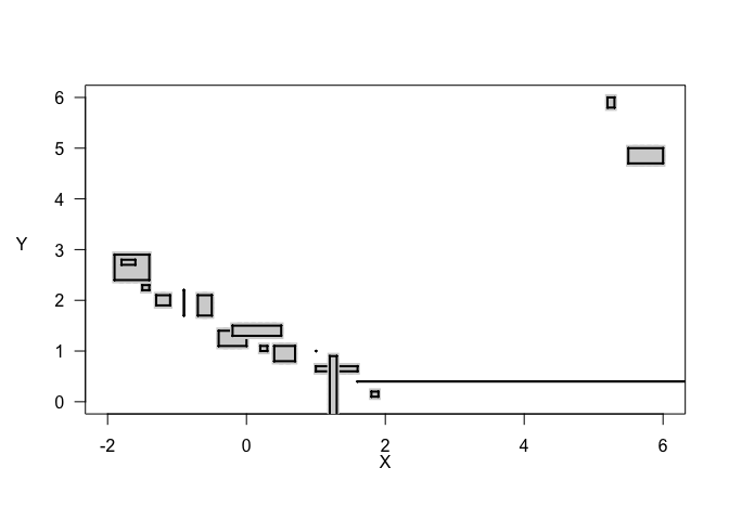
The likelihood-based imprecise regression method that we consider here is more limited in scope. In this method, we have data whose aleatoric, or measurement, uncertainty is expressed as an interval. This interval data might come from the precision of your measuring device or from binned survey data, for example. So, each data point is a set, rather than a point. A scatter plot of our interval data shows how the different sets can look. In the degenerate case, when both the x-value and y-value are known precisely, we have a single point, like traditional precise datasets. In the typical case, we have a square defined by the x-interval and the y-interval. Note that these sets can be overlapping or entirely contained within one another. Lastly, we also have cases where at least one interval is unbounded. This results in a line or a rectangle that extends infinitely in one direction. In the case of a line, one variable is known precisely but the other is not.

plot(data_idf, typ = "draft", k.x = 10, k.y = 10, p.cex = 1.5, y.las = 1, y.adj = 6)

Likelihood-based imprecise regression

The linLIR package is built specifically for simple linear regression, so we’ll be fitting the model $y=a+bx$ , using the imprecise data. Mirroring the set nature of the $x$ and $y$ variables, our estimates for $a$ and $b$ will also be set-valued.

Before we can estimate the slope and intercept, we need to set some parameters for the LIR method. We’ll call the s.linlir function to conduct the optimization. The syntax is s.linlir(dat.idf, var = NULL, p = 0.5, bet, epsilon = 0, a.grid = 100), let’s consider each input:

dat.idf is the interval data frame that contains our data. We created this in our previous step.

var is the variable names, which defaults to NULL. Since we’ve already labeled our variables, we’ll keep the default.

p is the quantile we are interested in estimating. The default value is set to the median, at 0.5. In standard least squares regression, we estimate the mean response. LIR uses quantile regression, where we estimate the median response (or any other quantile of interest).

bet is the $\beta$ value that controls the confidence level of our results. Setting $\beta = 0.5$ results in an asymptotically lower bounded confidence level of 76.1%. See Cattaneo and Wiencierz (2012) for more details on setting $\beta$ .

epsilon is the probability that a given interval-valued observation does not contain the true value. The default value is set to 0, indicating that all of the interval data contain the true values. While p and bet control the type of output we are interested in, epsilon is a parametric representation of reality. The value is typically set subjectively based on the analyst’s confidence in the data but in some cases quantitative information may be available based on past data or similar systems. Setting epsilon makes the assumption that $P(X_{\text{low}} \leq X \leq X_{\text{high}} \text{ and } Y_{\text{low}} \leq Y \leq Y_{\text{high}}) \geq 1-\epsilon$ .

a.grid is a parameter that controls the fineness of the approximation used to calculate the results. We’ll use the default.

To summarize, we’ll use our dataset, set $\beta = 0.5$ and take the default for the rest of the settings.

model_lir <- s.linlir(data_idf, bet = 0.5)
summary(model_lir)
## 
## Simple linear LIR analysis results 
## 
## Call:
## s.linlir(dat.idf = data_idf, bet = 0.5)
## 
## Ranges of parameter values of the undominated functions:
## intercept of f in [-0.1015873,2.600819]
## slope of f in [-2.051587,0.323809]
## 
## Bandwidth:  0.7619048 
## 
## Estimated parameters of the function f.lrm:
## intercept of f.lrm:  1.428571 
## slope of f.lrm:  -0.6190476 
## 
## Number of observations: 17 
## 
## LIR settings:
## p: 0.5    beta: 0.5    epsilon: 0    k.l: 6    k.u: 11  
## confidence level of each confidence interval: 76.21 %

Given these parameters, the goal of quantile regression is to determine the regression line that results in the smallest band containing the desired quantile of data points. In precise quantile regression, we use residuals to find this optimal function. In imprecise quantile regression, we consider the so-called lower and upper residuals, which are the distance between the regression line and the closest and furthest points of a given set-valued observation.

$\begin{align*} \mathcal{B} &:= \left\{\frac{\bar{y}_i-\bar{y}_j}{\underline{x}_i-\underline{x}_j} \,:\, (i, j) \in \mathcal{D}^2 \text{ and } \underline{x}_i > \underline{x}_j \text{ and }\bar{y}_i > \bar{y}_j \right\} \,\cup\, \\ & \left\{\frac{\underline{y}_i-\underline{y}_j}{\underline{x}_i-\underline{x}_j} \,:\, (i, j) \in \mathcal{D}^2 \text{ and } \underline{x}_i > \underline{x}_j \text{ and }\underline{y}_i < \underline{y}_j \right\} \,\cup\, \\ & \left\{\frac{\bar{y}_i-\bar{y}_j}{\bar{x}_i-\bar{x}_j} \,:\, (i, j) \in \mathcal{D}^2 \text{ and } \bar{x}_i > \bar{x}_j \text{ and }\bar{y}_i < \bar{y}_j \right\} \,\cup\, \\ & \left\{\frac{\underline{y}_i-\underline{y}_j}{\bar{x}_i-\bar{x}_j} \,:\, (i, j) \in \mathcal{D}^2 \text{ and } \bar{x}_i > \bar{x}_j \text{ and }\underline{y}_i > \underline{y}_j \right\} \,\cup\, \{0\} \end{align*}$

These lower and upper residuals will produce a set of regression lines, rather than a single line.

$\begin{align*} \underline{z}_{b,i} = \begin{cases} \underline{y}_i - b\underline{x}_i & \text{if } b < 0 \\ \underline{y} & \text{if } b = 0 \\ \underline{y}_i - b\bar{x}_i & \text{if } b > 0 \end{cases} \end{align*}$ $\begin{align*} \bar{z}_{b,i} = \begin{cases} \bar{y}_i - b\bar{x}_i & \text{if } b < 0 \\ \bar{y} & \text{if } b = 0 \\ \bar{y}_i - b\underline{x}_i & \text{if } b > 0 \end{cases} \end{align*}$

From this set, we’ll find the set of all undominated regression functions. We call a regression function undominated if no other function provides a better fit across all possible lower and upper residuals. Mathematically, we find this set by first finding smallest upper residual across all possible regression functions, $\bar{q}_{LRM} = \inf_{f \in F{\bar{r}_{f,(\bar{k})}}}$ , then take the set of all functions whose lower residual is less than or equal to that bound, $\mathcal{U} = \{f \in F : \underline{r}_{f,(\underline{k})} \leq \bar{q}_{LRM}\}$ . Combining these formulas with our explicit residuals, we have

$\begin{align*} \bar{q}_{LRM} &= \frac{1}{2} \min_{(b,j) \in \mathcal{B} \times \{1,\ldots,n-\bar{k}+1\}}{(\bar{z}_{b,[j]}-\underline{z}_{b,(j)})} \\ \mathcal{U} = \{f \in \mathcal{F} \,:\, \bar{r}_{f,(\bar{k})} = \bar{q}_{LRM}\} &\supseteq \{f_{a',b'} \,:\, (b',j') \in \text{argmin}_{(b,j) \in \mathcal{B} \times \{1,\ldots,n-\bar{k}+1\}}\{(\bar{z}_{b,[j]}-\underline{z}_{b,(j)})\} \\ & \text{ and } a' = \frac{1}{2} (\underline{z}_{b',(j')}+\bar{z}_{b',[j']}) \} \end{align*}$

This set of functions represents the statistical uncertainty from the finite sample (like precise regression) but also the measurement uncertainty from the imprecise data (unlike precise regression).

The good news: linLIR implements an algorithm that conducts this search and optimization process.

The bad news: the algorithmic complexity is $O(n^3\log{n})$ …which is very expensive and also why our sample set is only 17 observations! A sample size of 500 observations should take about an hour to run.

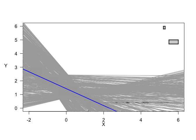
In this case, the set of undominated regression functions does not have a conclusively positive or negative slope, likely because of the outliers in the top right. However, our best estimate in blue, the likelihood-based region minimax (LRM) estimate (listed as “f.lrm” in the numeric results), agrees with the majority of undominated functions with a significant negative slope. Unlike confidence intervals in precise regression, note that our set of functions is not convex - there are spaces between some lines. This feature of imprecise regression is common when there is significant variation in the shape and spacing of the data. When the data are more homogenous and we have more samples, the result-set tends to approach a convex set, which resembles a traditional confidence interval. It is also important to note that this package randomly samples a subset of lines to display on the plot to restrict computation and graphics processing, which can also result in incorrectly displayed whitespace.

plot(model_lir, typ = "qlrm", lrm.col = "blue", pl.dat = TRUE, pl.dat.typ = "draft",
     k.x=10, k.y=10, y.las=1, y.adj=6)

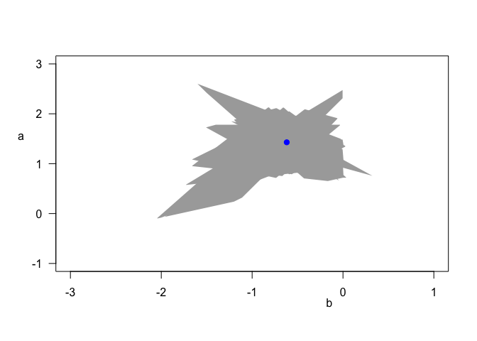
The non-convex nature of the results can also be seen directly in the parameter estimates, which have an unusual, jagged shape. Again the best estimate is highlighted in blue.

plot(model_lir, typ = "para", x.adj = 0.7, y.las = 1, y.adj = 6, y.padj = -3)

The graphical results here, and the numeric intervals presented earlier, emphasize the uncertainty that remains in our result. As you might have expected, the large uncertainty in our data has carried through to our results. The benefit is that we have quantified this uncertainty, numerically and visually, and can readily communicate it to a decision maker. In precise regression, we know that we have model misspecification risk, but it is difficult to know how much or how that compares among different models.

Other approaches

The major alternative approach to imprecise regression is to use “fuzzy” models. Typically these models are less general in that they make restrictive distributional assumptions on data and/or parameters. The benefit to using them is that the methods are more mature and well-known, e.g. the frbs package.

Another closely related approach is traditional sensitivity analysis. This is easy to implement, and conceptually very similar to the imprecise approach, but is necessarily limited in scope.

Exercises

Using the linLIR package load the pm10 dataset as an interval data frame (don’t forget to start with a clean session of R…no tidyverse). Extract the first 50 rows of the data and label the first variable as “Particulate Matter” and the second as “VO2 Max”. Particulate matter ( $PM_{10}$ ) is the standardized relative parts per million of coarse pollutants in the air, a measure of air quality. Maximal aerobic capacity ( $VO_2 \text{Max}$ ) is the maximal rate of oxygen uptake during exercise, a measure of fitness.

Plot $VO_2 \text{Max}$ by $PM_{10}$ . Which variable is measured more precisely?

(Note: this a notional interpretation of the toy variables in the package and does not reflect real data)
Fit a likelihood-based imprecise regression model predicting the 80th percentile of V02 Max by Particulate Matter. What are your interval estimates for the slope and intercept of the regression line?
Plot the undominated regression lines from your previous model. Give two possible explanations for the white space between the regression lines.
How does your confidence level change if you fit the 50th percentile instead? Why?

UC Business Analytics R Programming Guide