![]() Follow me on twitter @bradleyboehmke
Follow me on twitter @bradleyboehmke
![]() Follow me on twitter @bradleyboehmke
Follow me on twitter @bradleyboehmke
![]()
The Naïve Bayes classifier is a simple probabilistic classifier which is based on Bayes theorem but with strong assumptions regarding independence. Historically, this technique became popular with applications in email filtering, spam detection, and document categorization. Although it is often outperformed by other techniques, and despite the naïve design and oversimplified assumptions, this classifier can perform well in many complex real-world problems. And since it is a resource efficient algorithm that is fast and scales well, it is definitely a machine learning algorithm to have in your toolkit.
This tutorial serves as an introduction to the naïve Bayes classifier and covers:
caret package.h2o package.This tutorial leverages the following packages.
library(rsample)  # data splitting
library(dplyr)    # data transformation
library(ggplot2)  # data visualization
library(caret)    # implementing with caret
library(h2o)      # implementing with h2o
To illustrate the naïve Bayes classifier we will use the attrition data that has been included in the rsample package. The goal is to predict employee attrition.
# conver some numeric variables to factors
attrition <- attrition %>%
  mutate(
    JobLevel = factor(JobLevel),
    StockOptionLevel = factor(StockOptionLevel),
    TrainingTimesLastYear = factor(TrainingTimesLastYear)
  )

# Create training (70%) and test (30%) sets for the attrition data.
# Use set.seed for reproducibility
set.seed(123)
split <- initial_split(attrition, prop = .7, strata = "Attrition")
train <- training(split)
test  <- testing(split)

# distribution of Attrition rates across train & test set
table(train$Attrition) %>% prop.table()
##
##       No      Yes
## 0.838835 0.161165
table(test$Attrition) %>% prop.table()
##
##        No       Yes
## 0.8386364 0.1613636
The naïve Bayes classifier is founded on Bayesian probability, which originated from Reverend Thomas Bayes. Bayesian probability incorporates the concept of conditional probability, the probabilty of event A given that event B has occurred [denoted as ]. In the context of our attrition data, we are seeking the probability of an employee belonging to attrition class (where and ) given that its predictor values are . This can be written as .
The Bayesian formula for calculating this probability is
where:
is the prior probability of the outcome. Essentially, based on the historical data, what is the probability of an employee attriting or not. As we saw in the above section preparing our training and test sets, our prior probability of an employee attriting was about 16% and the probability of not attriting was about 84%.
is the probability of the predictor variables (same as ). Essentially, based on the historical data, what is the probability of each observed combination of predictor variables. When new data comes in, this becomes our evidence.
is the conditional probability or likelihood. Essentially, for each class of the response variable (i.e. attrit or not attrit), what is the probability of observing the predictor values.
is called our posterior probability. By combining our observed information, we are updating our a priori information on probabilities to compute a posterior probability that an observation has class .
We can re-write Eq. (1) in plain english as:
Although Eq. (1) has simplistic beauty on its surface, it becomes complex and intractable as the number of predictor variables grow. In fact, to compute the posterior probability for a response variable with m classes and a data set with p predictors, Eq. (1) would require probabilities computed. So for our attrition data, we have 2 classes (attrition vs. non-attrition) and 31 variables, requiring 2,147,483,648 probabilities computed.
Consequently, the naïve Bayes classifier makes a simplifying assumption (hence the name) to allow the computation to scale. With naïve Bayes, we assume that the predictor variables are conditionally independent of one another given the response value. This is an extremely strong assumption. We can see quickly that our attrition data violates this as we have several moderately to strongly correlated variables.
train %>%
  filter(Attrition == "Yes") %>%
  select_if(is.numeric) %>%
  cor() %>%
  corrplot::corrplot()
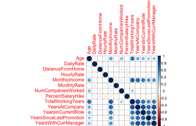
However, by making this assumption we can simplify our calculation such that the posterior probability is simply the product of the probability distribution for each individual variable conditioned on the response category (Eq. 2). Now we are only required to compute probabilities (this equates to 62 probabilities for our data set), a far more managable task.
For categorical variables, this computation is quite simple as you just use the frequencies from the data. However, when including continuous predictor variables often an assumption of normality is made so that we can use the probability from the variable’s probability density function. If we pick a handful of our numeric features we quickly see assumption of normality is not always fair.
train %>%
  select(Age, DailyRate, DistanceFromHome, HourlyRate, MonthlyIncome, MonthlyRate) %>%
  gather(metric, value) %>%
  ggplot(aes(value, fill = metric)) +
  geom_density(show.legend = FALSE) +
  facet_wrap(~ metric, scales = "free")

Granted, some numeric features may be normalized with a Box-Cox transformation; however, as you will see in this tutorial we can also use non-parametric kernel density estimators to try get a more accurate representation of continuous variable probabilities. Ultimately, transforming the distributions and selecting an estimator is part of the modeling development and tuning process.
One additional issue to be aware of - since naïve Bayes uses the product of feature probabilities conditioned on each class, we run into a serious problem when new data includes a feature value that never occurs for one or more levels of a response class. What results is for this individual feature and this zero will ripple through the entire multiplication of all features and will always force the posterior probability to be zero for that class.
A solution to this problem involves using the Laplace smoother. The Laplace smoother adds a small number to each of the counts in the frequencies for each feature, which ensures that each feature has a nonzero probability of occuring for each class. Typically, a value of one to two for the Laplace smoother is sufficient, but this is a tuning parameter to incorporate and optimize with cross validation.
The naïve Bayes classifier is simple (both intuitively and computationally), fast, performs well with small amounts of training data, and scales well to large data sets. The greatest weakness of the naïve Bayes classifier is that it relies on an often-faulty assumption of equally important and independent features which results in biased posterior probabilities. Although this assumption is rarely met, in practice, this algorithm works surprisingly well. This is primarily because what is usually needed is not a propensity (exact posterior probability) for each record that is accurate in absolute terms but just a reasonably accurate rank ordering of propensities.
For example, we may not care about the exact posterior probability of attrition, we just want to know for a given observation, is the posterior probability of attriting larger than not attriting. Even when the assumption is violated, the rank ordering of the records’ propensities is typically preserved. Consequentely, naïve Bayes is often a surprisingly accurate algorithm; however, on average it rarely can compete with the accuracy of advanced tree-based methods (random forests & gradient boosting machines) but is definitely worth having in your toolkit.
There are several packages to apply naïve Bayes (i.e. e1071, klaR, naivebayes, bnclassify). This tutorial demonstrates using the caret and h2o packages. caret allows us to use the different naïve Bayes packages above but in a common framework, and also allows for easy cross validation and tuning. h2o allows us to perform naïve Bayes in a powerful and scalable architecture.
caretFirst, we apply a naïve Bayes model with 10-fold cross validation, which gets 83% accuracy. Considering about 83% of our observations in our training set do not attrit, our overall accuracy is no better than if we just predicted “No” attrition for every observation.
# create response and feature data
features <- setdiff(names(train), "Attrition")
x <- train[, features]
y <- train$Attrition

# set up 10-fold cross validation procedure
train_control <- trainControl(
  method = "cv",
  number = 10
  )

# train model
nb.m1 <- train(
  x = x,
  y = y,
  method = "nb",
  trControl = train_control
  )

# results
confusionMatrix(nb.m1)
## Cross-Validated (10 fold) Confusion Matrix
##
## (entries are percentual average cell counts across resamples)
##
##           Reference
## Prediction   No  Yes
##        No  75.3  8.3
##        Yes  8.5  7.8
##
##  Accuracy (average) : 0.8311
We can tune the few hyperparameters that a naïve Bayes model has.
usekernel parameter allows us to use a kernel density estimate for continuous variables versus a guassian density estimate,adjust allows us to adjust the bandwidth of the kernel density (larger numbers mean more flexible density estimate),fL allows us to incorporate the Laplace smoother.If we just tuned our model with the above parameters we are able to lift our accuracy to 85%; however, by incorporating some preprocessing of our features (normalize with Box Cox, standardize with center-scaling, and reducing with PCA) we actually get about another 2% lift in our accuracy.
# set up tuning grid
search_grid <- expand.grid(
  usekernel = c(TRUE, FALSE),
  fL = 0:5,
  adjust = seq(0, 5, by = 1)
)

# train model
nb.m2 <- train(
  x = x,
  y = y,
  method = "nb",
  trControl = train_control,
  tuneGrid = search_grid,
  preProc = c("BoxCox", "center", "scale", "pca")
  )

# top 5 modesl
nb.m2$results %>%
  top_n(5, wt = Accuracy) %>%
  arrange(desc(Accuracy))
##   usekernel fL adjust  Accuracy     Kappa AccuracySD   KappaSD
## 1      TRUE  1      3 0.8737864 0.4435322 0.02858175 0.1262286
## 2      TRUE  0      2 0.8689320 0.4386202 0.02903618 0.1155707
## 3      TRUE  2      3 0.8689320 0.4750282 0.02830559 0.0970368
## 4      TRUE  2      4 0.8689320 0.4008608 0.02432572 0.1234943
## 5      TRUE  4      5 0.8689320 0.4439767 0.02867321 0.1354681

# plot search grid results
plot(nb.m2)
![]()
# results for best model
confusionMatrix(nb.m2)
## Cross-Validated (10 fold) Confusion Matrix
##
## (entries are percentual average cell counts across resamples)
##
##           Reference
## Prediction   No  Yes
##        No  80.8  9.5
##        Yes  3.1  6.6
##
##  Accuracy (average) : 0.8738
We can assess the accuracy on our final holdout test set. Its obvious that our model is not capturing a large percentage of our actual attritions (illustrated by our low specificity).
pred <- predict(nb.m2, newdata = test)
confusionMatrix(pred, test$Attrition)
## Confusion Matrix and Statistics
##
##           Reference
## Prediction  No Yes
##        No  349  41
##        Yes  20  30
##
##                Accuracy : 0.8614
##                  95% CI : (0.8255, 0.8923)
##     No Information Rate : 0.8386
##     P-Value [Acc > NIR] : 0.10756
##
##                   Kappa : 0.4183
##  Mcnemar's Test P-Value : 0.01045
##
##             Sensitivity : 0.9458
##             Specificity : 0.4225
##          Pos Pred Value : 0.8949
##          Neg Pred Value : 0.6000
##              Prevalence : 0.8386
##          Detection Rate : 0.7932
##    Detection Prevalence : 0.8864
##       Balanced Accuracy : 0.6842
##
##        'Positive' Class : No
##
h2oLets go ahead and start up h2o:
# start up h2o
h2o.no_progress()
h2o.init()
##
## H2O is not running yet, starting it now...
##
## Note:  In case of errors look at the following log files:
##     /var/folders/ws/qs4y2bnx1xs_4y9t0zbdjsvh0000gn/T//Rtmpfor8zk/h2o_bradboehmke_started_from_r.out
##     /var/folders/ws/qs4y2bnx1xs_4y9t0zbdjsvh0000gn/T//Rtmpfor8zk/h2o_bradboehmke_started_from_r.err
##
##
## Starting H2O JVM and connecting: ... Connection successful!
##
## R is connected to the H2O cluster:
##     H2O cluster uptime:         3 seconds 48 milliseconds
##     H2O cluster timezone:       America/New_York
##     H2O data parsing timezone:  UTC
##     H2O cluster version:        3.18.0.4
##     H2O cluster version age:    1 month and 11 days
##     H2O cluster name:           H2O_started_from_R_bradboehmke_tqs570
##     H2O cluster total nodes:    1
##     H2O cluster total memory:   1.78 GB
##     H2O cluster total cores:    4
##     H2O cluster allowed cores:  4
##     H2O cluster healthy:        TRUE
##     H2O Connection ip:          localhost
##     H2O Connection port:        54321
##     H2O Connection proxy:       NA
##     H2O Internal Security:      FALSE
##     H2O API Extensions:         XGBoost, Algos, AutoML, Core V3, Core V4
##     R Version:                  R version 3.4.4 (2018-03-15)
We can compute a naïve Bayes model in h2o with h2o.naiveBayes. Here we use the default model with no Laplace smoother. We experience similar results on our training cross validation as we did using caret.
# create feature names
y <- "Attrition"
x <- setdiff(names(train), y)

# h2o cannot ingest ordered factors
train.h2o <- train %>%
  mutate_if(is.factor, factor, ordered = FALSE) %>%
  as.h2o()

# train model
nb.h2o <- h2o.naiveBayes(
  x = x,
  y = y,
  training_frame = train.h2o,
  nfolds = 10,
  laplace = 0
)

# assess results
h2o.confusionMatrix(nb.h2o)
## Confusion Matrix (vertical: actual; across: predicted)  for max f1 @ threshold = 0.751627773135859:
##         No Yes    Error       Rate
## No     812  52 0.060185    =52/864
## Yes     77  89 0.463855    =77/166
## Totals 889 141 0.125243  =129/1030
We can also do some feature preprocessing as we did with caret and tune the Laplace smoother using h2o.grid. We don’t see much improvement.
# do a little preprocessing
preprocess <- preProcess(train, method = c("BoxCox", "center", "scale", "pca"))
train_pp   <- predict(preprocess, train)
test_pp    <- predict(preprocess, test)

# convert to h2o objects
train_pp.h2o <- train_pp %>%
  mutate_if(is.factor, factor, ordered = FALSE) %>%
  as.h2o()

test_pp.h2o <- test_pp %>%
  mutate_if(is.factor, factor, ordered = FALSE) %>%
  as.h2o()

# get new feature names --> PCA preprocessing reduced and changed some features
x <- setdiff(names(train_pp), "Attrition")

# create tuning grid
hyper_params <- list(
  laplace = seq(0, 5, by = 0.5)
  )

# build grid search
grid <- h2o.grid(
  algorithm = "naivebayes",
  grid_id = "nb_grid",
  x = x,
  y = y,
  training_frame = train_pp.h2o,
  nfolds = 10,
  hyper_params = hyper_params
  )

# Sort the grid models by mse
sorted_grid <- h2o.getGrid("nb_grid", sort_by = "accuracy", decreasing = TRUE)
sorted_grid
## H2O Grid Details
## ================
##
## Grid ID: nb_grid
## Used hyper parameters:
##   -  laplace
## Number of models: 11
## Number of failed models: 0
##
## Hyper-Parameter Search Summary: ordered by decreasing accuracy
##    laplace        model_ids           accuracy
## 1      2.5  nb_grid_model_5 0.8572815533980582
## 2      5.0 nb_grid_model_10 0.8572815533980582
## 3      3.0  nb_grid_model_6 0.8533980582524272
## 4      2.0  nb_grid_model_4 0.8504854368932039
## 5      1.5  nb_grid_model_3 0.8466019417475728
## 6      4.5  nb_grid_model_9 0.8407766990291262
## 7      0.5  nb_grid_model_1 0.8398058252427184
## 8      4.0  nb_grid_model_8 0.8339805825242719
## 9      3.5  nb_grid_model_7 0.8281553398058252
## 10     1.0  nb_grid_model_2 0.8194174757281554
## 11     0.0  nb_grid_model_0 0.8009708737864077

# grab top model id
best_h2o_model <- sorted_grid@model_ids[[1]]
best_model <- h2o.getModel(best_h2o_model)

# confusion matrix of best model
h2o.confusionMatrix(best_model)
## Confusion Matrix (vertical: actual; across: predicted)  for max f1 @ threshold = 0.402989172890541:
##         No Yes    Error       Rate
## No     796  68 0.078704    =68/864
## Yes     59 107 0.355422    =59/166
## Totals 855 175 0.123301  =127/1030

# ROC curve
auc <- h2o.auc(best_model, xval = TRUE)
fpr <- h2o.performance(best_model, xval = TRUE) %>% h2o.fpr() %>% .[['fpr']]
tpr <- h2o.performance(best_model, xval = TRUE) %>% h2o.tpr() %>% .[['tpr']]
data.frame(fpr = fpr, tpr = tpr) %>%
  ggplot(aes(fpr, tpr) ) +
  geom_line() +
  ggtitle( sprintf('AUC: %f', auc) )
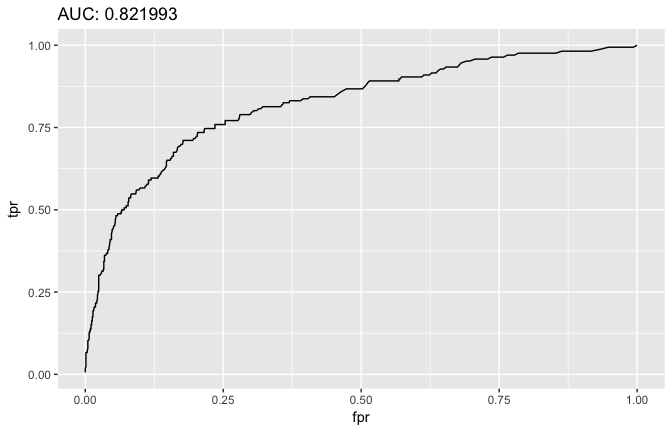
Once we’ve identified the optimal model we can assess on our test set.
# evaluate on test set
h2o.performance(best_model, newdata = test_pp.h2o)
## H2OBinomialMetrics: naivebayes
##
## MSE:  0.1001466
## RMSE:  0.3164595
## LogLoss:  0.334571
## Mean Per-Class Error:  0.2107714
## AUC:  0.8480667
## Gini:  0.6961334
##
## Confusion Matrix (vertical: actual; across: predicted) for F1-optimal threshold:
##         No Yes    Error     Rate
## No     307  62 0.168022  =62/369
## Yes     18  53 0.253521   =18/71
## Totals 325 115 0.181818  =80/440
##
## Maximum Metrics: Maximum metrics at their respective thresholds
##                         metric threshold    value idx
## 1                       max f1  0.271470 0.569892 113
## 2                       max f2  0.146349 0.672451 175
## 3                 max f0point5  0.590826 0.608856  48
## 4                 max accuracy  0.702382 0.875000  31
## 5                max precision  0.979861 1.000000   0
## 6                   max recall  0.000385 1.000000 399
## 7              max specificity  0.979861 1.000000   0
## 8             max absolute_mcc  0.539455 0.498232  57
## 9   max min_per_class_accuracy  0.219049 0.788618 132
## 10 max mean_per_class_accuracy  0.271470 0.789229 113
##
## Gains/Lift Table: Extract with `h2o.gainsLift(<model>, <data>)` or `h2o.gainsLift(<model>, valid=<T/F>, xval=<T/F>)`

# predict new data
h2o.predict(nb.h2o, newdata = test_pp.h2o)
##   predict        No         Yes
## 1      No 0.9851309 0.014869060
## 2      No 0.9109746 0.089025413
## 3      No 0.9947524 0.005247592
## 4      No 0.9694504 0.030549563
## 5      No 0.9683716 0.031628419
## 6      No 0.9836910 0.016308996
##
## [440 rows x 3 columns]

# shut down h2o
h2o.shutdown(prompt = FALSE)
## [1] TRUE
Although we did not see much improvement over the baseline response class proportions in this example, the naïve Bayes classifier is often hard to beat in terms of CPU and memory consumption as shown by Huang, J. (2003), and in certain cases its performance can be very close to more complicated and slower techniques. Consquently, its a solid technique to have in your toolkit. If you want to dig deeper into this classifier, I would start with: