![]() Follow me on twitter @bradleyboehmke
Follow me on twitter @bradleyboehmke
![]() Follow me on twitter @bradleyboehmke
Follow me on twitter @bradleyboehmke
 In this tutorial, you will learn general tools that are useful for many different forecasting situations. It will describe some methods for benchmark forecasting, methods for checking whether a forecasting model has adequately utilized the available information, and methods for measuring forecast accuracy. Each of the tools discussed in this tutorial will be used repeatedly in subsequent tutorials as you develop and explore a range of forecasting methods.
This tutorial serves as an introduction to basic benchmarking approaches for time series data and covers:
This tutorial leverages a variety of data sets to illustrate unique time series features. The data sets are all provided by the forecast and fpp2 packages. Furthermore, these packages provide various functions for computing and visualizing basic time series components.
library(forecast)
library(fpp2)
Although it is tempting to apply “sophisticated” forecasting methods, one must remember to consider naive forecasts. A naive forecast is simply the most recently observed value. In other words, at the time t, the k-step-ahead naive forecast () equals the observed value at time t ().
Sometimes, this is the best that can be done for many time series including most stock price data (for reasons illustrated in the previous tutorial’s exercise). Even if it is not a good forecasting method, it provides a useful benchmark for other forecasting methods. We can perform a naive forecast with the naive function.
Here, we use naive to forecast the next 10 values. The resulting output is an object of class forecast. This is the core class of objects in the forecast package, and there are many functions for dealing with them. We can print off the model summary with summary, which provides us with the residual standard deviation, some error measures (which we will cover later), and the actual forecasted values.
fc_goog <- naive(goog, 10)
summary(fc_goog)
##
## Forecast method: Naive method
##
## Model Information:
## Call: naive(y = goog, h = 10)
##
## Residual sd: 8.9145
##
## Error measures:
##                     ME     RMSE      MAE        MPE      MAPE MASE
## Training set 0.4436236 8.921089 6.008889 0.06493981 0.9815741    1
##                    ACF1
## Training set 0.04680557
##
## Forecasts:
##      Point Forecast    Lo 80    Hi 80    Lo 95    Hi 95
## 1001         838.96 827.5272 850.3928 821.4750 856.4450
## 1002         838.96 822.7915 855.1285 814.2325 863.6875
## 1003         838.96 819.1577 858.7623 808.6751 869.2449
## 1004         838.96 816.0943 861.8257 803.9900 873.9300
## 1005         838.96 813.3954 864.5246 799.8623 878.0577
## 1006         838.96 810.9554 866.9646 796.1306 881.7894
## 1007         838.96 808.7116 869.2084 792.6990 885.2210
## 1008         838.96 806.6231 871.2969 789.5049 888.4151
## 1009         838.96 804.6615 873.2585 786.5050 891.4150
## 1010         838.96 802.8062 875.1138 783.6675 894.2525
You will notice the forecast output provides a point forecast (the last observed value in the goog data set) and prediction confidence levels at the 80% and 95% level. A prediction interval gives an interval within which we expect to lie with a specified probability. For example, assuming the forecast errors are uncorrelated and normally distributed, then a simple 95% prediction interval for the next observation in a time series is
where is an estimate of the standard deviation of the forecast distribution. In forecasting, it is common to calculate 80% intervals and 95% intervals, although any percentage may be used.
When forecasting one-step ahead, the standard deviation of the forecast distribution is almost the same as the standard deviation of the residuals. (In fact, the two standard deviations are identical if there are no parameters to be estimated such as with the naive method. For forecasting methods involving parameters to be estimated, the standard deviation of the forecast distribution is slightly larger than the residual standard deviation, although this difference is often ignored.)
For example, consider our naive forecast for the goog data. The last value of the observed series is 838.96, so the forecast of the next value is 838.96 and the standard deviation of the residuals from the naive method is 8.91. Hence, a 95% prediction interval for the next value of goog is
Similarly, an 80% prediction interval is given by
The value of prediction intervals is that they express the uncertainty in the forecasts. If we only produce point forecasts, there is no way of telling how accurate the forecasts are. But if we also produce prediction intervals, then it is clear how much uncertainty is associated with each forecast. Thus, with the naive forecast on the next goog value, we can be 80% confident that the next value will be in the range of 828-850 and 95% confident that the the value will be between 821-856.
We can illustrate this prediction interval by plotting the naive model (fc_goog). Here, we see the black point estimate line flat-line (equal to the last observed value) and the colored bands represent our 80% and 95% prediction confidence interval. A common feature of prediction intervals is that they increase in length as the forecast horizon increases. The further ahead we forecast, the more uncertainty is associated with the forecast, and so the prediction intervals grow wider.1
# forecast next 25 values
fc_goog <- naive(goog, 25)

autoplot(fc_goog)

For seasonal data, a related idea is to use the corresponding season from the last year of data. For example, if you want to forecast the sales volume for next March, you would use the sales volume from the previous March. For a series with M seasons, we can write this as
This is implemented in the snaive function, meaning, seasonal naive. Here I use snaive to forecast the next 16 values for the ausbeer series. Here we see that the 4th quarter for each future year is 488 which is the last observed 4th quarter value in 2009.
fc_beer <- snaive(ausbeer, 16)
summary(fc_beer)
##
## Forecast method: Seasonal naive method
##
## Model Information:
## Call: snaive(y = ausbeer, h = 16)
##
## Residual sd: 19.1207
##
## Error measures:
##                    ME     RMSE      MAE      MPE    MAPE MASE       ACF1
## Training set 3.098131 19.32591 15.50935 0.838741 3.69567    1 0.01093868
##
## Forecasts:
##         Point Forecast    Lo 80    Hi 80    Lo 95    Hi 95
## 2010 Q3            419 394.2329 443.7671 381.1219 456.8781
## 2010 Q4            488 463.2329 512.7671 450.1219 525.8781
## 2011 Q1            414 389.2329 438.7671 376.1219 451.8781
## 2011 Q2            374 349.2329 398.7671 336.1219 411.8781
## 2011 Q3            419 383.9740 454.0260 365.4323 472.5677
## 2011 Q4            488 452.9740 523.0260 434.4323 541.5677
## 2012 Q1            414 378.9740 449.0260 360.4323 467.5677
## 2012 Q2            374 338.9740 409.0260 320.4323 427.5677
## 2012 Q3            419 376.1020 461.8980 353.3932 484.6068
## 2012 Q4            488 445.1020 530.8980 422.3932 553.6068
## 2013 Q1            414 371.1020 456.8980 348.3932 479.6068
## 2013 Q2            374 331.1020 416.8980 308.3932 439.6068
## 2013 Q3            419 369.4657 468.5343 343.2438 494.7562
## 2013 Q4            488 438.4657 537.5343 412.2438 563.7562
## 2014 Q1            414 364.4657 463.5343 338.2438 489.7562
## 2014 Q2            374 324.4657 423.5343 298.2438 449.7562
Similar to naive, we can plot the snaive model with autoplot.
autoplot(fc_beer)

When applying a forecasting method, it is important to always check that the residuals are well-behaved (i.e., no outliers or patterns) and resemble white noise. Essential assumptions for an appropriate forecasting model include residuals being:
Furthermore, the prediction intervals are computed assuming that the residuals:
A convenient function to use to check these assumptions is the checkresiduals function. This function produces a time plot, ACF plot, histogram, and a Ljung-Box test on the residuals. Here, I use checkresiduals for the fc_goog naive model. We see that the top plot shows residuals that appear to be white noise (no discernable pattern), the bottom left plot shows only a couple lags that exceed the 95% confidence interval, bottom right plot shows the residuals to be approximately normally distributed, and the Ljung-Box test results give a p-value of 0.22 suggesting the residuals are white noise. This is a good thing as it suggests that are model captures all (or most) of the available signal in the data.
checkresiduals(fc_goog)

##
## 	Ljung-Box test
##
## data:  residuals
## Q* = 13.061, df = 10, p-value = 0.2203
##
## Model df: 0.   Total lags used: 10
If we compare that to the fc_beer seasonal naive model we see that there is an apparent pattern in the residual time series plot, the ACF plot shows several lags exceeding the 95% confidence interval, and the Ljung-Box test has a statistically significant p-value suggesting the residuals are not purely white noise. This suggests that there may be another model or additional variables that will better capture the remaining signal in the data.
checkresiduals(fc_beer)

##
## 	Ljung-Box test
##
## data:  residuals
## Q* = 60.535, df = 8, p-value = 3.661e-10
##
## Model df: 0.   Total lags used: 8
A training set is a data set that is used to discover possible relationships. A test set is a data set that is used to verify the strength of these potential relationships. When you separate a data set into these parts, you generally allocate more of the data for training, and less for testing. There is one important difference between data partitioning in cross-sectional and time series data. In cross-sectional data the partitioning is usually done randomly, with a random set of observations designated as training data and the remainder as test data. However, in time series, a random partition creates two problems:
Therefore, time series partitioning into training and test sets is done by taking a training partition from earlier observations and then using a later partition for the test set.
One function that can be used to create training and test sets is subset.ts(), which returns a subset of a time series where the start and end of the subset are specified using index values. The gold time series comprises daily gold prices over 1108 trading days. Let’s use the first 1000 days as a training set. We can also create a test data set of the remaining data.
train <- subset.ts(gold, end = 1000)
test <- subset.ts(gold, start = 1001, end = length(gold))
A similar approach can be used for data where we want to maintain season features. For example, if we use subset.ts to take the first 1,000 observations this may include half of a year in the training data and the other half in the test data. Rather, for forecasting methods that include seasonal features (i.e. snaive), we prefer to not split a full cycle of seasons (i.e. year, month, week). We can use the window function to do this. For example, the ausbeer data set has quarterly data from 1956-2010. Here, we take data from 1956 through the 4th quarter of 1995 to be a training data set.
train2 <- window(ausbeer, end = c(1995, 4))
The window function is also particularly useful when we want to take data from a defined period. For example, if we decide that data from 1956-1969 is not appropriate due to regulatory changes then we can create a training data set from the 1st qtr of 1970 through the 4th qtr of 1995.
train3 <- window(ausbeer, start = c(1970, 1), end = c(1995, 4))
For evaluating predictive performance, several measures are commonly used to assess the predictive accuracy of a forecasting method. In all cases, the measures are based on the test data set, which serves as a more objective basis than the training period to assess predictive accuracy. Given a forecast and it’s given errors (), the commonly used accuracy measures are listed below:
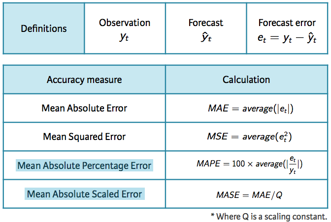
Forecast Accuracy Measures
Note that each measure has its strengths and weaknesses. For example, if you want to compare forecast accuracy between two series on very different scales you can’t compare the MAE or MSE for these forecast as these measures depend on the scale of the time series data. MAPE is often better for comparisons but only if our data are all positive and have no zeros or small values. It also assumes a natural zero so it can’t be used for temperature forecasts as these are based on arbitrary zero scales. MASE is similar to MAE but is scaled so that it can be compared across different data series. You can read more about each of these measures here; however, for now just keep in mind that for all these measures a smaller value signifies a better forecast.
We can compute all of these measures by using the accuracy function. The accuracy measures provided also include root mean squared error (RMSE) which is the square root of the mean squared error (MSE). Minimizing RMSE, which corresponds with increasing accuracy, is the same as minimizing MSE. In addition, other accuracy measures not illustrated above are also provided (i.e. ACF1 - autocorrelation at lag 1; Theil’s U). The output of accuracy allows us to compare these accuracy measures for the residuals of the training data set against the forecast errors of the test data. However, our main concern is how well different forecasting methods improve the predictive accuracy on the test data.
Using the training data we created from the gold data set (train), let’s create two different forecasts:
naive forecast andHere, I use h = 108 to predict for the next 108 days (note that the gold data set has 1108 observations, the training data set has 1000, so we want to predict the next 108 observations and compare that to the test data.).
# create training data
train <- subset.ts(gold, end = 1000)

# Compute naive forecasts and save to naive_fc
naive_fc <- naive(train, h = 108)

# Compute mean forecasts and save to mean_fc
mean_fc <- meanf(train, h = 108)

# Use accuracy() to compute forecast accuracy
accuracy(naive_fc, gold)
##                       ME     RMSE       MAE         MPE     MAPE MASE
## Training set  0.09161392  6.33977  3.158386  0.01662141 0.794523    1
## Test set     -6.53834951 15.84236 13.638350 -1.74622688 3.428789   NA
##                    ACF1 Theil's U
## Training set -0.3098928        NA
## Test set      0.9793153  5.335899
accuracy(mean_fc, gold)
##                         ME     RMSE      MAE       MPE      MAPE     MASE
## Training set -4.239671e-15 59.17809 53.63397 -2.390227 14.230224 16.98145
## Test set      1.319363e+01 19.55255 15.66875  3.138577  3.783133       NA
##                   ACF1 Theil's U
## Training set 0.9907254        NA
## Test set     0.9793153  6.123788
What accuracy is doing is taking the model output from the training data (naive_fc & mean_fc) and computing the accuracy measures of the 108 forecasted values to those values in gold that are not included in the model (aka test data). This means we do not need to directly feed it a test data set, although we do have that option as illustrated below:
train <- subset.ts(gold, end = 1000)
test <- subset.ts(gold, start = 1001, end = length(gold))
naive_fc <- naive(train, h = 108)
accuracy(naive_fc, test)
##                       ME     RMSE       MAE         MPE     MAPE MASE
## Training set  0.09161392  6.33977  3.158386  0.01662141 0.794523    1
## Test set     -6.53834951 15.84236 13.638350 -1.74622688 3.428789   NA
##                    ACF1 Theil's U
## Training set -0.3098928        NA
## Test set      0.9793153  5.335899
If we compare the test set accuracy measures for both models we see that the naive approach has lower scores across all measures indicating better forecasting accuracy.
We can use a similar approach to evaluate the accuracy of seasonal forecasting models. The primary difference is we want to use the window function for creating our training data so that we appropriately capture seasonal cycles. Here, I illustrate with the ausbeer data set. We see the snaive model produces lower scores across all measures indicating better forecasting accuracy.
# create training data
train2 <- window(ausbeer, end = c(1995, 4))

# create specific test data of interest
test <- window(ausbeer, start = c(1996, 1), end = c(2004, 4))

# Compute snaive forecasts and save to snaive_fc
snaive_fc <- snaive(train2, h = length(test))

# Compute mean forecasts and save to mean_fc
mean_fc <- meanf(train2, h = length(test))

# Use accuracy() to compute forecast accuracy
accuracy(snaive_fc, test)
##                     ME     RMSE      MAE       MPE     MAPE      MASE
## Training set  4.730769 20.60589 16.51282  1.284697 3.957622 1.0000000
## Test set     -8.527778 18.06854 13.08333 -2.011727 3.038430 0.7923137
##                     ACF1 Theil's U
## Training set  0.01783674        NA
## Test set     -0.39101873 0.2890478
accuracy(mean_fc, test)
##                         ME     RMSE      MAE       MPE      MAPE     MASE
## Training set -2.279427e-14 96.37835 78.64437 -6.646984 21.996740 4.762625
## Test set      2.393472e+01 49.38745 34.07500  4.640789  7.243654 2.063548
##                     ACF1 Theil's U
## Training set  0.72972747        NA
## Test set     -0.09479634 0.8164006
A more sophisticated version of training/test sets is cross-validation. You can see how cross-validation works for cross-sectional data here. For time series data, the procedure is similar but the training set consists only of observations that occurred prior to the observation that forms the test set. So in traditional time series partitioning, we select a certain point in time where everything before that point (blue) is the training data and everything after that point (red) is the test data.
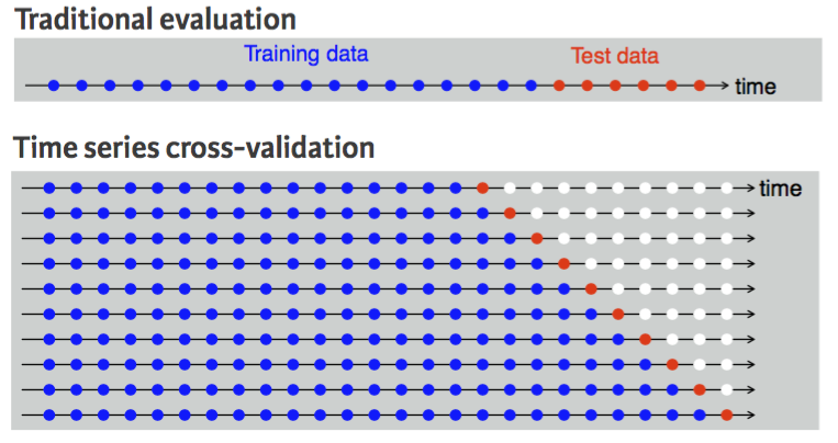
Time Series Cross-Validation
However, assuming we want to perform a 1-step forecast (predicting the next value in the series), time series cross-validation will:
This procedure is sometimes known as a “rolling forecasting origin” because the “origin” () at which the forecast is based rolls forward in time as displayed by each row in the above illustration.
With time series forecasting, one-step forecasts may not be as relevant as multi-step forecasts. In this case, the cross-validation procedure based on a rolling forecasting origin can be modified to allow multi-step errors to be used. Suppose we are interested in models that produce good h-step-ahead forecasts. Here, we simply adjust the above algorithm so that we select the observation at time for the test set, use the observations at times to estimate the forecasting model, compute the h-step error on the forecast for time , rinse & repeat until we can compute the forecasting accuracy for all errors calculated. For a 2-step-ahead forecast this looks like:
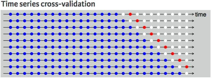
Two-Step Ahead Time Series Cross-Validation
This seems tedious, however, there is a simple function that implements this procedure. The tsCV function applies a forecasting model to a sequence of training sets from a given time series and provides the errors as the output. However, we need to compute our own accuracy measures with these errors.
As an example, let’s perform a cross-validation approach for a 1-step ahead (h=1) naive model with the goog data. We can then compute the MSE which is 79.59.
errors <- tsCV(goog, forecastfunction = naive, h = 1)
mean(errors^2, na.rm = TRUE)
## [1] 79.58582
We can compute and compare the MSE for different forecast horizons (1-10) to see if certain forecasting horizons perform better than others. Here, we see that as the forecasting horizon extends the predictive accuracy becomes poorer.
# create empty vector to hold MSE values
MSE <- vector("numeric", 10)
for(h in 1:10) {
  errors <- tsCV(goog, forecastfunction = naive, h = h)
  MSE[h] <- mean(errors^2, na.rm = TRUE)
}

MSE
##  [1]  79.58582 167.14427 253.92996 330.20539 398.47090 464.83012 531.09256
##  [8] 596.40191 654.25322 712.70988
Using the built-in AirPassengers data set:
AirPassengers data set, perform a time series cross validation that:
There are some exceptions to this. For example, some non-linear forecasting methods do not have this attribute. ↩