![]() Follow me on twitter @bradleyboehmke
Follow me on twitter @bradleyboehmke
![]() Follow me on twitter @bradleyboehmke
Follow me on twitter @bradleyboehmke
So far we’ve analyzed the Harry Potter series by understanding the frequency and distribution of words across the corpus. This can be useful in giving context of particular text along with understanding the general sentiment. However, we often want to understand the relationship between words in a corpus. What sequences of words are common across our text? Given a sequence of words, what word is most likely to follow? What words have the strongest relationship with each other? These are questions that we will consider in this tutorial.
This tutorial builds on the tidy text, sentiment analysis, and term vs. document frequency tutorials so if you have not read through those tutorials I suggest you start there before proceeding. In this tutorial I cover the following:
This tutorial leverages the data provided in the harrypotter package. I constructed this package to supply the first seven novels in the Harry Potter series to illustrate text mining and analysis capabilities. You can load the harrypotter package with the following:
if (packageVersion("devtools") < 1.6) {
  install.packages("devtools")
}

devtools::install_github("bradleyboehmke/harrypotter")
library(tidyverse)      # data manipulation & plotting
library(stringr)        # text cleaning and regular expressions
library(tidytext)       # provides additional text mining functions
library(harrypotter)    # provides the first seven novels of the Harry Potter series
The seven novels we are working with, and are provided by the harrypotter package, include:
philosophers_stone: Harry Potter and the Philosophers Stone (1997)chamber_of_secrets: Harry Potter and the Chamber of Secrets (1998)prisoner_of_azkaban: Harry Potter and the Prisoner of Azkaban (1999)goblet_of_fire: Harry Potter and the Goblet of Fire (2000)order_of_the_phoenix: Harry Potter and the Order of the Phoenix (2003)half_blood_prince: Harry Potter and the Half-Blood Prince (2005)deathly_hallows: Harry Potter and the Deathly Hallows (2007)Each text is in a character vector with each element representing a single chapter. For instance, the following illustrates the raw text of the first two chapters of the philosophers_stone:
philosophers_stone[1:2]
## [1] "THE BOY WHO LIVED  Mr. and Mrs. Dursley, of number four, Privet Drive, were proud to say that they
## were perfectly normal, thank you very much. They were the last people you'd expect to be involved in anything
## strange or mysterious, because they just didn't hold with such nonsense.  Mr. Dursley was the director of a
## firm called Grunnings, which made drills. He was a big, beefy man with hardly any neck, although he did have a
## very large mustache. Mrs. Dursley was thin and blonde and had nearly twice the usual amount of neck, which came
## in very useful as she spent so much of her time craning over garden fences, spying on the neighbors. The
## Dursleys had a small son called Dudley and in their opinion there was no finer boy anywhere.  The Dursleys
## had everything they wanted, but they also had a secret, and their greatest fear was that somebody would
## discover it. They didn't think they could bear it if anyone found out about the Potters. Mrs. Potter was Mrs.
## Dursley's sister, but they hadn'... <truncated>
## [2] "THE VANISHING GLASS  Nearly ten years had passed since the Dursleys had woken up to find their nephew on
## the front step, but Privet Drive had hardly changed at all. The sun rose on the same tidy front gardens and lit
## up the brass number four on the Dursleys' front door; it crept into their living room, which was almost exactly
## the same as it had been on the night when Mr. Dursley had seen that fateful news report about the owls. Only
## the photographs on the mantelpiece really showed how much time had passed. Ten years ago, there had been lots
## of pictures of what looked like a large pink beach ball wearing different-colored bonnets -- but Dudley Dursley
## was no longer a baby, and now the photographs showed a large blond boy riding his first bicycle, on a carousel
## at the fair, playing a computer game with his father, being hugged and kissed by his mother. The room held no
## sign at all that another boy lived in the house, too.  Yet Harry Potter was still there, asleep at the
## moment, but no... <truncated>
As we saw in the tidy text, sentiment analysis, and term vs. document frequency tutorials we can use the unnest function from the tidytext package to break up our text by words, paragraphs, etc. We can also use unnest to break up our text by “tokens”, aka - a consecutive sequence of words. These are commonly referred to as n-grams where a bi-gram is a pair of two consecutive words, a tri-gram is a group of three consecutive words, etc.
Here, we follow the same process to prepare our text as we have in the previous three tutorials; however, notice that in the unnest function I apply a token argument to state we want n-grams and the n = 2 tells it we want bi-grams.
titles <- c("Philosopher's Stone", "Chamber of Secrets", "Prisoner of Azkaban",
            "Goblet of Fire", "Order of the Phoenix", "Half-Blood Prince",
            "Deathly Hallows")

books <- list(philosophers_stone, chamber_of_secrets, prisoner_of_azkaban,
           goblet_of_fire, order_of_the_phoenix, half_blood_prince,
           deathly_hallows)

series <- tibble()

for(i in seq_along(titles)) {

        clean <- tibble(chapter = seq_along(books[[i]]),
                        text = books[[i]]) %>%
             unnest_tokens(bigram, text, token = "ngrams", n = 2) %>%
             mutate(book = titles[i]) %>%
             select(book, everything())

        series <- rbind(series, clean)
}

# set factor to keep books in order of publication
series$book <- factor(series$book, levels = rev(titles))

series
## # A tibble: 1,089,186 × 3
##                   book chapter      bigram
## *               <fctr>   <int>       <chr>
## 1  Philosopher's Stone       1     the boy
## 2  Philosopher's Stone       1     boy who
## 3  Philosopher's Stone       1   who lived
## 4  Philosopher's Stone       1    lived mr
## 5  Philosopher's Stone       1      mr and
## 6  Philosopher's Stone       1     and mrs
## 7  Philosopher's Stone       1 mrs dursley
## 8  Philosopher's Stone       1  dursley of
## 9  Philosopher's Stone       1   of number
## 10 Philosopher's Stone       1 number four
## # ... with 1,089,176 more rows
Our output is similar to what we had in the previous tutorials; however, note that our bi-grams have groups of two words. Also, note how there is some repetition, or overlapping. The sentence “The boy who lived” is broken up into 3 bi-grams:
This is done for the entire Harry Potter series and captures all the sequences of two consecutive words. We can now perform common frequency analysis procedures. First, let’s look at the most common bi-grams across the entire Harry Potter series:
series %>%
        count(bigram, sort = TRUE)
## # A tibble: 340,021 × 2
##        bigram     n
##         <chr> <int>
## 1      of the  4895
## 2      in the  3571
## 3  said harry  2626
## 4      he was  2490
## 5      at the  2435
## 6      to the  2386
## 7      on the  2359
## 8      he had  2138
## 9      it was  2123
## 10     out of  1911
## # ... with 340,011 more rows
With the exception of “said harry” the most common bi-grams include very common words that do not provide much context. We can filter out these common stop words to find the most common bi-grams that provide context. The results show pairs of words that are far more contextual than our previous set.
series %>%
        separate(bigram, c("word1", "word2"), sep = " ") %>%
        filter(!word1 %in% stop_words$word,
               !word2 %in% stop_words$word) %>%
        count(word1, word2, sort = TRUE)
## Source: local data frame [89,120 x 3]
## Groups: word1 [14,752]
##
##           word1      word2     n
##           <chr>      <chr> <int>
## 1     professor mcgonagall   578
## 2         uncle     vernon   386
## 3         harry     potter   349
## 4         death     eaters   346
## 5         harry     looked   316
## 6         harry        ron   302
## 7          aunt    petunia   206
## 8  invisibility      cloak   192
## 9     professor  trelawney   177
## 10         dark       arts   176
## # ... with 89,110 more rows
Similar to the previous text mining tutorials we can visualize the top 10 bi-grams for each book.
series %>%
        separate(bigram, c("word1", "word2"), sep = " ") %>%
        filter(!word1 %in% stop_words$word,
               !word2 %in% stop_words$word) %>%
        count(book, word1, word2, sort = TRUE) %>%
        unite("bigram", c(word1, word2), sep = " ") %>%
        group_by(book) %>%
        top_n(10) %>%
        ungroup() %>%
        mutate(book = factor(book) %>% forcats::fct_rev()) %>%
        ggplot(aes(drlib::reorder_within(bigram, n, book), n, fill = book)) +
        geom_bar(stat = "identity", alpha = .8, show.legend = FALSE) +
        drlib::scale_x_reordered() +
        facet_wrap(~ book, ncol = 2, scales = "free") +
        coord_flip()

We can also follow a similar process as performed in the term vs. document frequency tutorial to identify the tf-idf of n-grams (or bi-grams in our ongoing example).
(bigram_tf_idf <- series %>%
        count(book, bigram, sort = TRUE) %>%
        bind_tf_idf(bigram, book, n) %>%
        arrange(desc(tf_idf))
)
## Source: local data frame [523,420 x 6]
## Groups: book [7]
##
##                    book             bigram     n           tf       idf
##                  <fctr>              <chr> <int>        <dbl>     <dbl>
## 1        Goblet of Fire          mr crouch   152 0.0007923063 1.2527630
## 2     Half-Blood Prince      said slughorn    84 0.0004904995 1.9459101
## 3   Prisoner of Azkaban    professor lupin   107 0.0010165981 0.8472979
## 4  Order of the Phoenix professor umbridge   173 0.0006686636 1.2527630
## 5       Deathly Hallows                c i    83 0.0004173602 1.9459101
## 6       Deathly Hallows              c but    62 0.0003117630 1.9459101
## 7       Deathly Hallows          the elder    60 0.0003017061 1.9459101
## 8       Deathly Hallows         elder wand    58 0.0002916493 1.9459101
## 9    Chamber of Secrets      said lockhart    38 0.0004450587 1.2527630
## 10  Prisoner of Azkaban         said lupin    97 0.0009215889 0.5596158
## # ... with 523,410 more rows, and 1 more variables: tf_idf <dbl>
And we can visualize the bigrams with the highest tf_idf for each book:
bigram_tf_idf %>%
        group_by(book) %>%
        top_n(15, wt = tf_idf) %>%
        ungroup() %>%
        mutate(book = factor(book) %>% forcats::fct_rev()) %>%
        ggplot(aes(drlib::reorder_within(bigram, tf_idf, book), tf_idf, fill = book)) +
        geom_bar(stat = "identity", alpha = .8, show.legend = FALSE) +
        labs(title = "Highest tf-idf bi-grams in the Harry Potter series",
             x = NULL, y = "tf-idf") +
        drlib::scale_x_reordered() +
        facet_wrap(~book, ncol = 2, scales = "free") +
        coord_flip()

The sentiment analysis approch used in the sentiment analysis tutorial simply counted the appearance of positive or negative words, according to a specified lexicon (i.e. AFINN, bing, nrc). Unfortunately, this approach scores the sentiments of words merely on their presence rather than on context. For example, the words “happy” and “like” will be counted as positive, even in a sentence like “I’m not happy and I don’t like it!”
By performing sentiment analysis on our bi-gram data, we can examine how often sentiment-associated words are preceded by “not” or other negating words.
series %>%
        separate(bigram, c("word1", "word2"), sep = " ") %>%
        filter(word1 == "not") %>%
        count(book, word1, word2, sort = TRUE)
## Source: local data frame [2,106 x 4]
## Groups: book, word1 [7]
##
##                    book word1 word2     n
##                  <fctr> <chr> <chr> <int>
## 1  Order of the Phoenix   not    to    90
## 2     Half-Blood Prince   not    to    79
## 3       Deathly Hallows   not    to    77
## 4        Goblet of Fire   not    to    45
## 5     Half-Blood Prince   not    be    42
## 6  Order of the Phoenix   not    be    39
## 7  Order of the Phoenix   not  have    37
## 8       Deathly Hallows   not    be    35
## 9       Deathly Hallows   not  know    35
## 10   Chamber of Secrets   not    to    34
## # ... with 2,096 more rows
We could use this to ignore or even reverse their contribution to the sentiment score. Here we’ll use the AFINN lexicon for the sentiment analysis, which gives a numeric sentiment score for each word. We can assess the most frequent words that have a sentiment score and were preceded by “not”.
AFINN <- get_sentiments("afinn")

(nots <- series %>%
        separate(bigram, c("word1", "word2"), sep = " ") %>%
        filter(word1 == "not") %>%
        inner_join(AFINN, by = c(word2 = "word")) %>%
        count(word2, score, sort = TRUE)
)
## Source: local data frame [201 x 3]
## Groups: word2 [201]
##
##     word2 score     n
##     <chr> <int> <int>
## 1    want     1    81
## 2    help     2    45
## 3    like     2    29
## 4    care     2    22
## 5     bad    -3    14
## 6    wish     1    14
## 7  stupid    -2    12
## 8    stop    -1    11
## 9  matter     1    10
## 10   dead    -3     9
## # ... with 191 more rows
We can use this information to see the total impact these cases had on misspecifying sentiment. For example, above we saw that the top two words preceded by “not” was “want” and “help”. The sentiment score for “want” is +1; however, “want” was preceded by “not” 81 times which means the sentiment could easily have been overstated by points. “help” on the otherhand has a sentiment score of +2 but was preceded by “not” 45 times which means the sentiment could have been overstated by points for these instances.
nots %>%
        mutate(contribution = n * score) %>%
        arrange(desc(abs(contribution))) %>%
        head(20) %>%
        ggplot(aes(reorder(word2, contribution), n * score, fill = n * score > 0)) +
        geom_bar(stat = "identity", show.legend = FALSE) +
        xlab("Words preceded by 'not'") +
        ylab("Sentiment score * # of occurrances") +
        coord_flip()
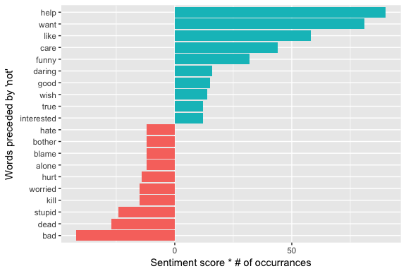
The bi-grams “not help”, “not want”, “not like” were the largest causes of misidentification, making the text seem much more positive than it is. We also see bi-grams such as “not bad”, “not dead”, and “not stupid” at the bottom of our chart suggesting these bi-grams made the text appear more negative than it is.
We could expand this example and use a full list of words that signal negation (i.e. “not”, “no”, “never”, “without”). This would allow us to find a larger pool of words that are preceded by negation and identify their impact on sentiment analysis.
negation_words <- c("not", "no", "never", "without")

(negated <- series %>%
                separate(bigram, c("word1", "word2"), sep = " ") %>%
                filter(word1 %in% negation_words) %>%
                inner_join(AFINN, by = c(word2 = "word")) %>%
                count(word1, word2, score, sort = TRUE) %>%
                ungroup()
)
## # A tibble: 379 × 4
##    word1   word2 score     n
##    <chr>   <chr> <int> <int>
## 1    not    want     1    81
## 2     no      no    -1    74
## 3     no   doubt    -1    53
## 4    not    help     2    45
## 5     no    good     3    38
## 6    not    like     2    29
## 7     no  chance     2    22
## 8    not    care     2    22
## 9     no problem    -2    21
## 10    no  matter     1    19
## # ... with 369 more rows
negated %>%
        mutate(contribution = n * score) %>%
        arrange(desc(abs(contribution))) %>%
        group_by(word1) %>%
        top_n(10, abs(contribution)) %>%
        ggplot(aes(drlib::reorder_within(word2, contribution, word1), contribution, fill = contribution > 0)) +
        geom_bar(stat = "identity", show.legend = FALSE) +
        xlab("Words preceded by 'not'") +
        ylab("Sentiment score * # of occurrances") +
        drlib::scale_x_reordered() +
        facet_wrap(~ word1, scales = "free") +
        coord_flip()

So far we’ve been visualizing the top n-grams; however, this doesn’t give us much insight into multiple relationships that exist among words. To get a better understanding of the numerous relationships that can exist we can use a network graph. First, we’ll set up the network structure using the igraph package. Here we’ll only focus on context words and look at bi-grams that have at least 20 occurrences across the entire Harry Potter series.
library(igraph)

(bigram_graph <- series %>%
        separate(bigram, c("word1", "word2"), sep = " ") %>%
        filter(!word1 %in% stop_words$word,
               !word2 %in% stop_words$word) %>%
        count(word1, word2, sort = TRUE) %>%
        unite("bigram", c(word1, word2), sep = " ") %>%
        filter(n > 20) %>%
        graph_from_data_frame()
)
## IGRAPH DN-- 375 291 --
## + attr: name (v/c)
## + edges (vertex names):
##  [1] professor mcgonagall->578 uncle vernon        ->386
##  [3] harry potter        ->349 death eaters        ->346
##  [5] harry looked        ->316 harry ron           ->302
##  [7] aunt petunia        ->206 invisibility cloak  ->192
##  [9] professor trelawney ->177 dark arts           ->176
## [11] professor umbridge  ->174 death eater         ->164
## [13] entrance hall       ->145 madam pomfrey       ->145
## [15] dark lord           ->141 professor dumbledore->127
## + ... omitted several edges
Now to visualize our network we’ll leverage the ggraph package which converts an igraph object to a ggplot-like graphich.
library(ggraph)
set.seed(123)

a <- grid::arrow(type = "closed", length = unit(.15, "inches"))

ggraph(bigram_graph, layout = "fr") +
        geom_edge_link() +
        geom_node_point(color = "lightblue", size = 5) +
        geom_node_text(aes(label = name), vjust = 1, hjust = 1) +
        theme_void()
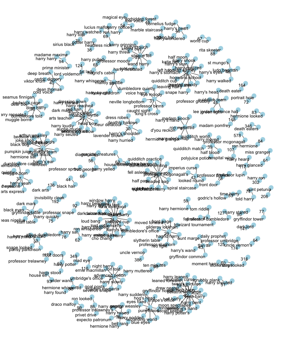
Here we can see clusters of word networks most commonly used together.
In addition to understanding what words and sentiments occur within sections, chapters, and books, we may also want to understand which pairs of words co-appear within sections, chapters, and books. Here we’ll focus on the philosophers_stone book.
(ps_words <- tibble(chapter = seq_along(philosophers_stone),
                  text = philosophers_stone) %>%
        unnest_tokens(word, text) %>%
        filter(!word %in% stop_words$word))
## # A tibble: 28,585 × 2
##    chapter      word
##      <int>     <chr>
## 1        1       boy
## 2        1     lived
## 3        1   dursley
## 4        1    privet
## 5        1     drive
## 6        1     proud
## 7        1 perfectly
## 8        1    normal
## 9        1    people
## 10       1    expect
## # ... with 28,575 more rows
We can leverage the widyr package to count common pairs of words co-appearing within the same chapter:
library(widyr)

(word_pairs <- ps_words %>%
        pairwise_count(word, chapter, sort = TRUE))
## # A tibble: 9,035,616 × 3
##     item1 item2     n
##     <chr> <chr> <dbl>
## 1   found  time    17
## 2    left  time    17
## 3    head  time    17
## 4     day  time    17
## 5     sat  time    17
## 6    eyes  time    17
## 7   heard  time    17
## 8   harry  time    17
## 9  looked  time    17
## 10   door  time    17
## # ... with 9,035,606 more rows
The output provids the pairs of words as two variables (item1 and item2). This allows us to perform normal text mining activities like looking for what words most often follow “harry”
word_pairs %>%
        filter(item1 == "harry")
## # A tibble: 5,420 × 3
##    item1  item2     n
##    <chr>  <chr> <dbl>
## 1  harry   time    17
## 2  harry  found    17
## 3  harry   left    17
## 4  harry   head    17
## 5  harry    day    17
## 6  harry    sat    17
## 7  harry   eyes    17
## 8  harry  heard    17
## 9  harry looked    17
## 10 harry   door    17
## # ... with 5,410 more rows
However, the most common co-appearing words only tells us part of the story. We may also want to know how often words appear together relative to how often they appear separately, or the correlation among words. Regarding text, correlation among words is measured in a binary form - either the words appear together or they do not. A common measure for such binary correlation is the phi coefficient.
Consider the following table:
| Has word Y | No word Y | Total | ||
|---|---|---|---|---|
| Has word X | ||||
| No word X | ||||
| Total | n |
For example, represents the number of documents where both word X and word Y appear, the number where neither appears, and and the cases where one appears without the other. In terms of this table, the phi coefficient is:
The pairwise_cor() function in widyr lets us find the correlation between words based on how often they appear in the same section. Its syntax is similar to pairwise_count().
(word_cor <- ps_words %>%
   group_by(word) %>%
   filter(n() >= 20) %>%
   pairwise_cor(word, chapter) %>%
   filter(!is.na(correlation)))
## # A tibble: 53,130 × 3
##       item1 item2 correlation
##       <chr> <chr>       <dbl>
## 1   dursley   boy  0.29880715
## 2     drive   boy  0.01543033
## 3    people   boy -0.16137431
## 4   strange   boy  0.87400737
## 5    called   boy  0.16499158
## 6  dursleys   boy  0.60385964
## 7    dudley   boy  0.68465320
## 8    potter   boy  0.16499158
## 9    street   boy  0.29880715
## 10   reason   boy -0.01543033
## # ... with 53,120 more rows
Similar to before we can now assess correlation for words of interest. For instance, what is the highest correlated words that appears with “potter”? Interestingly, it isn’t “harry”.
word_cor %>%
  filter(item1 == "potter") %>%
  arrange(desc(correlation))
## # A tibble: 230 × 3
##     item1    item2 correlation
##     <chr>    <chr>       <dbl>
## 1  potter    stood   0.6846532
## 2  potter    front   0.6846532
## 3  potter   moment   0.6846532
## 4  potter happened   0.6582806
## 5  potter     idea   0.4944132
## 6  potter    speak   0.4364358
## 7  potter  neville   0.4364358
## 8  potter standing   0.4333333
## 9  potter   stared   0.4333333
## 10 potter     fell   0.4333333
## # ... with 220 more rows
Similar to how we used ggraph to visualize bigrams, we can use it to visualize the correlations within word clusters. Here we look networks of words where the correlation is fairly high (> .65). We can see several clusters pop out. For instance, in the bottom right of the plot a cluster shows that “dursley”, “dudley”, “vernon”, “aunt”, “uncle”, “petunia”, “wizard”, and a few others are more likely to appear together than not. This type of graph provides a great starting point to find content relationships within text.
set.seed(123)

ps_words %>%
  group_by(word) %>%
  filter(n() >= 20) %>%
  pairwise_cor(word, chapter) %>%
  filter(!is.na(correlation),
         correlation > .65) %>%
  graph_from_data_frame() %>%
  ggraph(layout = "fr") +
  geom_edge_link(aes(edge_alpha = correlation), show.legend = FALSE) +
  geom_node_point(color = "lightblue", size = 5) +
  geom_node_text(aes(label = name), repel = TRUE) +
  theme_void()
