![]() Follow me on twitter @bradleyboehmke
Follow me on twitter @bradleyboehmke
![]() Follow me on twitter @bradleyboehmke
Follow me on twitter @bradleyboehmke
In the previous tutorial you learned that logistic regression is a classification algorithm traditionally limited to only two-class classification problems (i.e. default = Yes or No). However, if you have more than two classes then Linear (and its cousin Quadratic) Discriminant Analysis (LDA & QDA) is an often-preferred classification technique. Discriminant analysis models the distribution of the predictors X separately in each of the response classes (i.e. default = “Yes”, default = “No” ), and then uses Bayes’ theorem to flip these around into estimates for the probability of the response category given the value of X.
This tutorial serves as an introduction to LDA & QDA and covers1:
This tutorial primarily leverages the Default data provided by the ISLR package. This is a simulated data set containing information on ten thousand customers such as whether the customer defaulted, is a student, the average balance carried by the customer and the income of the customer. We’ll also use a few packages that provide data manipulation, visualization, pipeline modeling functions, and model output tidying functions.
# Packages
library(tidyverse)  # data manipulation and visualization
library(MASS)       # provides LDA & QDA model functions

# Load data
(default <- as_tibble(ISLR::Default))
## # A tibble: 10,000 × 4
##    default student   balance    income
##     <fctr>  <fctr>     <dbl>     <dbl>
## 1       No      No  729.5265 44361.625
## 2       No     Yes  817.1804 12106.135
## 3       No      No 1073.5492 31767.139
## 4       No      No  529.2506 35704.494
## 5       No      No  785.6559 38463.496
## 6       No     Yes  919.5885  7491.559
## 7       No      No  825.5133 24905.227
## 8       No     Yes  808.6675 17600.451
## 9       No      No 1161.0579 37468.529
## 10      No      No    0.0000 29275.268
## # ... with 9,990 more rows
In the previous tutorial we saw that a logistic regression model does a fairly good job classifying customers that default. So why do we need another classification method beyond logistic regression? There are several reasons:
However, its important to note that LDA & QDA have assumptions that are often more restrictive then logistic regression:
Also, when considering between LDA & QDA its important to know that LDA is a much less flexible classifier than QDA, and so has substantially lower variance. This can potentially lead to improved prediction performance. But there is a trade-off: if LDA’s assumption that the the predictor variable share a common variance across each Y response class is badly off, then LDA can suffer from high bias. Roughly speaking, LDA tends to be a better bet than QDA if there are relatively few training observations and so reducing variance is crucial. In contrast, QDA is recommended if the training set is very large, so that the variance of the classifier is not a major concern, or if the assumption of a common covariance matrix is clearly untenable.
As we’ve done in the previous tutorials, we’ll split our data into a training (60%) and testing (40%) data sets so we can assess how well our model performs on an out-of-sample data set.
set.seed(123)
sample <- sample(c(TRUE, FALSE), nrow(default), replace = T, prob = c(0.6,0.4))
train <- default[sample, ]
test <- default[!sample, ]
LDA computes “discriminant scores” for each observation to classify what response variable class it is in (i.e. default or not default). These scores are obtained by finding linear combinations of the independent variables. For a single predictor variable the LDA classifier is estimated as
where:
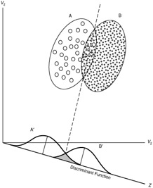
This classifier assigns an observation to the kth class of for which discriminant score () is largest. For example, lets assume there are two classes (A and B) for the response variable Y. Based on the predictor variable(s), LDA is going to compute the probability distribution of being classified as class A or B. The linear decision boundary between the probability distributions is represented by the dashed line. Discriminant scores to the left of the dashed line will be classified as A and scores to the right will be classified as B.
When dealing with more than one predictor variable, the LDA classifier assumes that the observations in the kth class are drawn from a multivariate Gaussian distribution , where is a class-specific mean vector, and is a covariance matrix that is common to all K classes. Incorporating this into the LDA classifier results in
where an observation will be assigned to class k where the discriminant score is largest.
In R, we fit a LDA model using the lda function, which is part of the MASS library. Notice that the syntax for the lda is identical to that of lm (as seen in the linear regression tutorial), and to that of glm (as seen in the logistic regression tutorial) except for the absence of the family option.
(lda.m1 <- lda(default ~ balance + student, data = train))
## Call:
## lda(default ~ balance + student, data = train)
##
## Prior probabilities of groups:
##        No       Yes
## 0.9677526 0.0322474
##
## Group means:
##      balance studentYes
## No   804.968  0.2956254
## Yes 1776.971  0.3948718
##
## Coefficients of linear discriminants:
##                     LD1
## balance     0.002232368
## studentYes -0.227922283
The LDA output indicates that our prior probabilities are and ; in other words, 96.8% of the training observations are customers who did not default and 3% represent those that defaulted. It also provides the group means; these are the average of each predictor within each class, and are used by LDA as estimates of . These suggest that customers that tend to default have, on average, a credit card balance of $1,777 and are more likely to be students then non-defaulters (29% of non-defaulters are students whereas 39% of defaulters are). However, as we learned from the last tutorial this is largely because students tend to have higher balances then non-students.
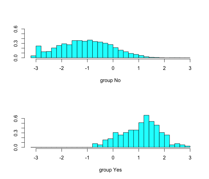
The coefficients of linear discriminants output provides the linear combination of balance and student=Yes that are used to form the LDA decision rule. In other words, these are the multipliers of the elements of X = x in Eq 1 & 2. If 0.0022 × balance − 0.228 × student is large, then the LDA classifier will predict that the customer will default, and if it is small, then the LDA classifier will predict the customer will not default. We can use plot to produce plots of the linear discriminants, obtained by computing 0.0022 × balance − 0.228 × student for each of the training observations. As you can see, when the probability increases that the customer will not default and when the probability increases that the customer will default.
plot(lda.m1)
We can use predict for LDA much like we did with logistic regression. I’ll illustrate the output that predict provides based on this simple data set.
(df <- tibble(balance = rep(c(1000, 2000), 2),
       student = c("No", "No", "Yes", "Yes")))
## # A tibble: 4 × 2
##   balance student
##     <dbl>   <chr>
## 1    1000      No
## 2    2000      No
## 3    1000     Yes
## 4    2000     Yes
Below we see that predict returns a list with three elements. The first element, class, contains LDA’s predictions about the customer defaulting. Here we see that the second observation (non-student with balance of $2,000) is the only one that is predicted to default. The second element, posterior, is a matrix that contains the posterior probability that the corresponding observations will or will not default. Here we see that the only observation to have a posterior probability of defaulting greater than 50% is observation 2, which is why the LDA model predicted this observation will default. However, we also see that observation 4 has a 42% probability of defaulting. Right now the model is predicting that this observation will not default because this probability is less than 50%; however, we will see shortly how we can make adjustments to our posterior probability thresholds. Finally, x contains the linear discriminant values, described earlier.
(df.pred <- predict(lda.m1, df))
## $class
## [1] No  Yes No  No
## Levels: No Yes
##
## $posterior
##          No         Yes
## 1 0.9903138 0.009686200
## 2 0.4585630 0.541436990
## 3 0.9940401 0.005959891
## 4 0.5801226 0.419877403
##
## $x
##         LD1
## 1 0.4335197
## 2 2.6658881
## 3 0.2055974
## 4 2.4379658
As previously mentioned the default setting is to use a 50% threshold for the posterior probabilities. We can recreate the predictions contained in the class element above:
# number of non-defaulters
sum(df.pred$posterior[, 1] >= .5)
## [1] 3

# number of defaulters
sum(df.pred$posterior[, 2] > .5)
## [1] 1
If we wanted to use a posterior probability threshold other than 50% in order to make predictions, then we could easily do so. For instance, suppose that a credit card company is extremely risk-adverse and wants to assume that a customer with 40% or greater probability is a high-risk customer. We can easily assess the number of high-risk customers.
# number of high-risk customers with 40% probability of defaulting
sum(df.pred$posterior[, 2] > .4)
## [1] 2
As previously mentioned, LDA assumes that the observations within each class are drawn from a multivariate Gaussian distribution and the covariance of the predictor variables are common across all k levels of the response variable Y. Quadratic discriminant analysis (QDA) provides an alternative approach. Like LDA, the QDA classifier assumes that the observations from each class of Y are drawn from a Gaussian distribution. However, unlike LDA, QDA assumes that each class has its own covariance matrix. In other words, the predictor variables are not assumed to have common variance across each of the k levels in Y. Mathematically, it assumes that an observation from the kth class is of the form , where is a covariance matrix for the kth class. Under this assumption, the classifier assigns an observation to the class for which
is largest. Why is this important? Consider the image below. In trying to classify the observations into the three (color-coded) classes, LDA (left plot) provides linear decision boundaries that are based on the assumption that the observations vary consistently across all classes. However, when looking at the data it becomes apparent that the variability of the observations within each class differ. Consequently, QDA (right plot) is able to capture the differing covariances and provide more accurate non-linear classification decision boundaries.
Similar to lda, we can use the MASS library to fit a QDA model. Here we use the qda function. The output is very similar to the lda output. It contains the prior probabilities and the group means. But it does not contain the coefficients of the linear discriminants, because the QDA classifier involves a quadratic, rather than a linear, function of the predictors.
(qda.m1 <- qda(default ~ balance + student, data = train))
## Call:
## qda(default ~ balance + student, data = train)
##
## Prior probabilities of groups:
##        No       Yes
## 0.9677526 0.0322474
##
## Group means:
##      balance studentYes
## No   804.968  0.2956254
## Yes 1776.971  0.3948718
The predict function works in exactly the same fashion as for LDA except it does not return the linear discriminant values. In comparing this simple prediction example to that seen in the LDA section we see minor changes in the posterior probabilities. Most notably, the posterior probability that observation 4 will default increased by nearly 8% points.
predict(qda.m1, df)
## $class
## [1] No  Yes No  No
## Levels: No Yes
##
## $posterior
##          No         Yes
## 1 0.9957697 0.004230299
## 2 0.4381383 0.561861660
## 3 0.9980862 0.001913799
## 4 0.5148050 0.485194962
Now that we understand the basics of evaluating our model and making predictions. Let’s assess how well our two models (lda.m1 & qda.m1) perform on our test data set. First we need to apply our models to the test data.
test.predicted.lda <- predict(lda.m1, newdata = test)
test.predicted.qda <- predict(qda.m1, newdata = test)
Now we can evaluate how well our model predicts by assessing the different classification rates discussed in the logistic regression tutorial. First we’ll look at the confusion matrix in a percentage form. The below results show that the models perform in a very similar manner. 96% of the predicted observations are true negatives and about 1% are true positives. Both models have a type II error of less than 3% in which the model predicts the customer will not default but they actually did. And both models have a type I error of less than 1% in which the models predict the customer will default but they never did.
lda.cm <- table(test$default, test.predicted.lda$class)
qda.cm <- table(test$default, test.predicted.qda$class)

list(LDA_model = lda.cm %>% prop.table() %>% round(3),
     QDA_model = qda.cm %>% prop.table() %>% round(3))
## $LDA_model
##
##          No   Yes
##   No  0.964 0.002
##   Yes 0.028 0.007
##
## $QDA_model
##
##          No   Yes
##   No  0.963 0.002
##   Yes 0.026 0.009
Furthermore, we can estimate the overall error rates. Here we see that the QDA model reduces the error rate by just a hair.
test %>%
  mutate(lda.pred = (test.predicted.lda$class),
         qda.pred = (test.predicted.qda$class)) %>%
  summarise(lda.error = mean(default != lda.pred),
            qda.error = mean(default != qda.pred))
## # A tibble: 1 × 2
##    lda.error  qda.error
##        <dbl>      <dbl>
## 1 0.02909183 0.02782697
However, as we discussed in the last tutorial, the overall error may be less important then understanding the precision of our model. If we look at the raw numbers of our confusion matrix we can compute the precision:
So our QDA model has a slightly higher precision than the LDA model; however, both of them are lower than the logistic regression model precision of 29%.
list(LDA_model = lda.cm,
     QDA_model = qda.cm)
## $LDA_model
##
##         No  Yes
##   No  3809    6
##   Yes  109   29
##
## $QDA_model
##
##         No  Yes
##   No  3808    7
##   Yes  103   35
If we are concerned with increasing the precision of our model we can tune our model by adjusting the posterior probability threshold. For instance, we might label any customer with a posterior probability of default above 20% as high-risk. Now the precision of our QDA model improves to . However, the overall error rate has increased to 4%. But a credit card company may consider this slight increase in the total error rate to be a small price to pay for more accurate identification of individuals who do indeed default. It’s important to keep in mind these kinds of trade-offs, which are common with classification models - tuning models can improve certain classification rates while worsening others.
# create adjusted predictions
lda.pred.adj <- ifelse(test.predicted.lda$posterior[, 2] > .20, "Yes", "No")
qda.pred.adj <- ifelse(test.predicted.qda$posterior[, 2] > .20, "Yes", "No")

# create new confusion matrices
list(LDA_model = table(test$default, lda.pred.adj),
     QDA_model = table(test$default, qda.pred.adj))
## $LDA_model
##      lda.pred.adj
##         No  Yes
##   No  3731   84
##   Yes   69   69
##
## $QDA_model
##      qda.pred.adj
##         No  Yes
##   No  3699  116
##   Yes   55   83
We can also assess the ROC curve for our models as we did in the logistic regression tutorial and compute the AUC.
# ROC curves
library(ROCR)

par(mfrow=c(1, 2))

prediction(test.predicted.lda$posterior[,2], test$default) %>%
  performance(measure = "tpr", x.measure = "fpr") %>%
  plot()

prediction(test.predicted.qda$posterior[,2], test$default) %>%
  performance(measure = "tpr", x.measure = "fpr") %>%
  plot()
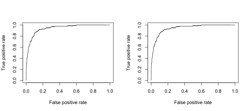
# model 1 AUC
prediction(test.predicted.lda$posterior[,2], test$default) %>%
  performance(measure = "auc") %>%
  .@y.values
## [[1]]
## [1] 0.9420727

# model 2 AUC
prediction(test.predicted.qda$posterior[,2], test$default) %>%
  performance(measure = "auc") %>%
  .@y.values
## [[1]]
## [1] 0.9420746
The logistic regression and LDA methods are closely connected and differ primarily in their fitting procedures. Consequently, the two often produce similar results. However, LDA assumes that the observations are drawn from a Gaussian distribution with a common covariance matrix across each class of Y, and so can provide some improvements over logistic regression when this assumption approximately holds. Conversely, logistic regression can outperform LDA if these Gaussian assumptions are not met. Both LDA and logistic regression produce linear decision boundaries so when the true decision boundaries are linear, then the LDA and logistic regression approaches will tend to perform well. QDA, on the other-hand, provides a non-linear quadratic decision boundary. Thus, when the decision boundary is moderately non-linear, QDA may give better results (we’ll see other non-linear classifiers in later tutorials).
What is important to keep in mind is that no one method will dominate the oth- ers in every situation. And often, we want to compare multiple approaches to see how they compare. To illustrate, we’ll examine stock market (Smarket) data provided by the ISLR package. This data set consists of percentage returns for the S&P 500 stock index over 1,250 days, from the beginning of 2001 until the end of 2005. For each date, percentage returns for each of the five previous trading days, Lag1 through Lag5 are provided. In addition Volume (the number of shares traded on the previous day, in billions), Today (the percentage return on the date in question) and Direction (whether the market was Up or Down on this date) are provided.
head(ISLR::Smarket)
##   Year   Lag1   Lag2   Lag3   Lag4   Lag5 Volume  Today Direction
## 1 2001  0.381 -0.192 -2.624 -1.055  5.010 1.1913  0.959        Up
## 2 2001  0.959  0.381 -0.192 -2.624 -1.055 1.2965  1.032        Up
## 3 2001  1.032  0.959  0.381 -0.192 -2.624 1.4112 -0.623      Down
## 4 2001 -0.623  1.032  0.959  0.381 -0.192 1.2760  0.614        Up
## 5 2001  0.614 -0.623  1.032  0.959  0.381 1.2057  0.213        Up
## 6 2001  0.213  0.614 -0.623  1.032  0.959 1.3491  1.392        Up
Lets model this data with logistic regression, LDA, and QDA to assess well each model does in predicting the direction of the stock market based on previous day returns. We’ll use 2001-2004 data to train our models and then test these models on 2005 data.
train <- subset(ISLR::Smarket, Year < 2005)
test <- subset(ISLR::Smarket, Year == 2005)
Here we fit a logistic regression model to the training data. Looking at the summary our model does not look too convincing considering no coefficients are statistically significant and our residual deviance has barely been reduced.
glm.fit <- glm(Direction ~ Lag1 + Lag2 + Lag3 + Lag4 + Lag5 + Volume,
               data = train,
               family = binomial)

summary(glm.fit)
##
## Call:
## glm(formula = Direction ~ Lag1 + Lag2 + Lag3 + Lag4 + Lag5 +
##     Volume, family = binomial, data = train)
##
## Deviance Residuals:
##    Min      1Q  Median      3Q     Max
## -1.302  -1.190   1.079   1.160   1.350
##
## Coefficients:
##              Estimate Std. Error z value Pr(>|z|)
## (Intercept)  0.191213   0.333690   0.573    0.567
## Lag1        -0.054178   0.051785  -1.046    0.295
## Lag2        -0.045805   0.051797  -0.884    0.377
## Lag3         0.007200   0.051644   0.139    0.889
## Lag4         0.006441   0.051706   0.125    0.901
## Lag5        -0.004223   0.051138  -0.083    0.934
## Volume      -0.116257   0.239618  -0.485    0.628
##
## (Dispersion parameter for binomial family taken to be 1)
##
##     Null deviance: 1383.3  on 997  degrees of freedom
## Residual deviance: 1381.1  on 991  degrees of freedom
## AIC: 1395.1
##
## Number of Fisher Scoring iterations: 3
Now we compute the predictions for 2005 and compare them to the actual movements of the market over that time period with a confusion matrix. The results are rather disappointing: the test error rate is 52%, which is worse than random guessing! Furthermore, our precision is only 31%. However, this should not be surprising considering the lack of statistical significance with our predictors.
# predictions
glm.probs <- predict(glm.fit, test, type="response")

# confusion matrix
table(test$Direction, ifelse(glm.probs > 0.5, "Up", "Down"))
##
##        Down Up
##   Down   77 34
##   Up     97 44

# accuracy rate
mean(ifelse(glm.probs > 0.5, "Up", "Down") == test$Direction)
## [1] 0.4801587

# error rate
mean(ifelse(glm.probs > 0.5, "Up", "Down") != test$Direction)
## [1] 0.5198413
Remember that using predictors that have no relationship with the response tends to cause a deterioration in the test error rate (since such predictors cause an increase in variance without a corresponding decrease in bias), and so removing such predictors may in turn yield an improvement. The variables that appear to have the highest importance rating are Lag1 and Lag2.
caret::varImp(glm.fit)
##           Overall
## Lag1   1.04620896
## Lag2   0.88432632
## Lag3   0.13941784
## Lag4   0.12456821
## Lag5   0.08257344
## Volume 0.48517564
Lets re-fit with just these two variables and reassess performance. We don’t see much improvement within our model summary.
glm.fit <- glm(Direction ~ Lag1 + Lag2,
               data = train,
               family = binomial)

summary(glm.fit)
##
## Call:
## glm(formula = Direction ~ Lag1 + Lag2, family = binomial, data = train)
##
## Deviance Residuals:
##    Min      1Q  Median      3Q     Max
## -1.345  -1.188   1.074   1.164   1.326
##
## Coefficients:
##             Estimate Std. Error z value Pr(>|z|)
## (Intercept)  0.03222    0.06338   0.508    0.611
## Lag1        -0.05562    0.05171  -1.076    0.282
## Lag2        -0.04449    0.05166  -0.861    0.389
##
## (Dispersion parameter for binomial family taken to be 1)
##
##     Null deviance: 1383.3  on 997  degrees of freedom
## Residual deviance: 1381.4  on 995  degrees of freedom
## AIC: 1387.4
##
## Number of Fisher Scoring iterations: 3
However, our prediction classification rates have improved slightly. Our error rate has decreased to 44% (accuracy = 56%) and our precision has increased to 75%. However, its worth noting that the market moved up 56% of the time in 2005 and moved down 44% of the time. Thus, the logistic regression approach is no better than a naive approach!
# predictions
glm.probs <- predict(glm.fit, test, type = "response")

# confusion matrix
table(test$Direction, ifelse(glm.probs > 0.5, "Up", "Down"))
##
##        Down  Up
##   Down   35  76
##   Up     35 106

# accuracy rate
mean(ifelse(glm.probs > 0.5, "Up", "Down") == test$Direction)
## [1] 0.5595238

# error rate
mean(ifelse(glm.probs > 0.5, "Up", "Down") != test$Direction)
## [1] 0.4404762
Now we’ll perform LDA on the stock market data. Our summary shows that our prior probabilities of market movement are 49% (down) and 51% (up). The group means indicate that there is a tendency for the previous 2 days’ returns to be negative on days when the market increases, and a tendency for the previous days’ returns to be positive on days when the market declines.
(lda.fit <- lda(Direction ~ Lag1 + Lag2, data = train))
## Call:
## lda(Direction ~ Lag1 + Lag2, data = train)
##
## Prior probabilities of groups:
##     Down       Up
## 0.491984 0.508016
##
## Group means:
##             Lag1        Lag2
## Down  0.04279022  0.03389409
## Up   -0.03954635 -0.03132544
##
## Coefficients of linear discriminants:
##             LD1
## Lag1 -0.6420190
## Lag2 -0.5135293
When we predict with our LDA model and assess the confusion matrix we see that our prediction rates mirror those produced by logistic regression. The overall error and the precision of our LDA and logistic regression models are the same.
# predictions
test.predicted.lda <- predict(lda.fit, newdata = test)

# confusion matrix
table(test$Direction, test.predicted.lda$class)
##
##        Down  Up
##   Down   35  76
##   Up     35 106

# accuracy rate
mean(test.predicted.lda$class == test$Direction)
## [1] 0.5595238

# error rate
mean(test.predicted.lda$class != test$Direction)
## [1] 0.4404762
Lastly, we’ll predict with a QDA model to see if we can improve our performance.
(qda.fit <- qda(Direction ~ Lag1 + Lag2, data = train))
## Call:
## qda(Direction ~ Lag1 + Lag2, data = train)
##
## Prior probabilities of groups:
##     Down       Up
## 0.491984 0.508016
##
## Group means:
##             Lag1        Lag2
## Down  0.04279022  0.03389409
## Up   -0.03954635 -0.03132544
Surprisingly, the QDA predictions are accurate almost 60% of the time! Furthermore, the precision of the model is 86%. This level of accuracy is quite impressive for stock market data, which is known to be quite hard to model accurately. This suggests that the quadratic form assumed by QDA may capture the true relationship more accurately than the linear forms assumed by LDA and logistic regression.
# predictions
test.predicted.qda <- predict(qda.fit, newdata = test)

# confusion matrix
table(test$Direction, test.predicted.qda$class)
##
##        Down  Up
##   Down   30  81
##   Up     20 121

# accuracy rate
mean(test.predicted.qda$class == test$Direction)
## [1] 0.5992063

# error rate
mean(test.predicted.qda$class != test$Direction)
## [1] 0.4007937
We can see how our models differ with a ROC curve. Although you can’t tell, the logistic regression and LDA ROC curves sit directly on top of one another. However, we can see how the QDA (green) differs slightly.
# ROC curves
library(ROCR)

p1 <- prediction(glm.probs, test$Direction) %>%
  performance(measure = "tpr", x.measure = "fpr")

p2 <- prediction(test.predicted.lda$posterior[,2], test$Direction) %>%
  performance(measure = "tpr", x.measure = "fpr")

p3 <- prediction(test.predicted.qda$posterior[,2], test$Direction) %>%
  performance(measure = "tpr", x.measure = "fpr")

plot(p1, col = "red")
plot(p2, add = TRUE, col = "blue")
plot(p3, add = TRUE, col = "green")
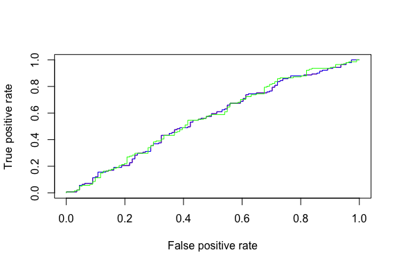
The difference is subtle. You can see where we experience increases in the true positive predictions (where the green line go above the red and blue lines). And although our precision increases, overall AUC is not that much higher.
# Logistic regression AUC
prediction(glm.probs, test$Direction) %>%
  performance(measure = "auc") %>%
  .@y.values
## [[1]]
## [1] 0.5584308

# LDA AUC
prediction(test.predicted.lda$posterior[,2], test$Direction) %>%
  performance(measure = "auc") %>%
  .@y.values
## [[1]]
## [1] 0.5584308

# QDA AUC
prediction(test.predicted.qda$posterior[,2], test$Direction) %>%
  performance(measure = "auc") %>%
  .@y.values
## [[1]]
## [1] 0.5620088
Although we get some improvement with the QDA model we probably want to continue tuning our models or assess other techniques to improve our classification performance before hedging any bets! But this illustrates the usefulness of assessing multiple classification models.
This will get you up and running with LDA and QDA. Keep in mind that there is a lot more you can dig into so the following resources will help you learn more:
This tutorial was built as a supplement to chapter 4, section 4 of An Introduction to Statistical Learning ↩