![]() Follow me on twitter @bradleyboehmke
Follow me on twitter @bradleyboehmke
![]() Follow me on twitter @bradleyboehmke
Follow me on twitter @bradleyboehmke
Clustering is a broad set of techniques for finding subgroups of observations within a data set. When we cluster observations, we want observations in the same group to be similar and observations in different groups to be dissimilar. Because there isn’t a response variable, this is an unsupervised method, which implies that it seeks to find relationships between the observations without being trained by a response variable. Clustering allows us to identify which observations are alike, and potentially categorize them therein. K-means clustering is the simplest and the most commonly used clustering method for splitting a dataset into a set of k groups.
This tutorial serves as an introduction to the k-means clustering method.
To replicate this tutorial’s analysis you will need to load the following packages:
library(tidyverse)  # data manipulation
library(cluster)    # clustering algorithms
library(factoextra) # clustering algorithms & visualization
To perform a cluster analysis in R, generally, the data should be prepared as follows:
Here, we’ll use the built-in R data set USArrests, which contains statistics in arrests per 100,000 residents for assault, murder, and rape in each of the 50 US states in 1973. It includes also the percent of the population living in urban areas
df <- USArrests
To remove any missing value that might be present in the data, type this:
df <- na.omit(df)
As we don’t want the clustering algorithm to depend to an arbitrary variable unit, we start by scaling/standardizing the data using the R function scale:
df <- scale(df)
head(df)
##                Murder   Assault   UrbanPop         Rape
## Alabama    1.24256408 0.7828393 -0.5209066 -0.003416473
## Alaska     0.50786248 1.1068225 -1.2117642  2.484202941
## Arizona    0.07163341 1.4788032  0.9989801  1.042878388
## Arkansas   0.23234938 0.2308680 -1.0735927 -0.184916602
## California 0.27826823 1.2628144  1.7589234  2.067820292
## Colorado   0.02571456 0.3988593  0.8608085  1.864967207
The classification of observations into groups requires some methods for computing the distance or the (dis)similarity between each pair of observations. The result of this computation is known as a dissimilarity or distance matrix. There are many methods to calculate this distance information; the choice of distance measures is a critical step in clustering. It defines how the similarity of two elements (x, y) is calculated and it will influence the shape of the clusters.
The choice of distance measures is a critical step in clustering. It defines how the similarity of two elements (x, y) is calculated and it will influence the shape of the clusters. The classical methods for distance measures are Euclidean and Manhattan distances, which are defined as follow:
Euclidean distance:
Manhattan distance:
Where, x and y are two vectors of length n.
Other dissimilarity measures exist such as correlation-based distances, which is widely used for gene expression data analyses. Correlation-based distance is defined by subtracting the correlation coefficient from 1. Different types of correlation methods can be used such as:
Pearson correlation distance:
Spearman correlation distance:
The spearman correlation method computes the correlation between the rank of x and the rank of y variables.
Where and .
Kendall correlation distance:
Kendall correlation method measures the correspondence between the ranking of x and y variables. The total number of possible pairings of x with y observations is n(n − 1)/2, where n is the size of x and y. Begin by ordering the pairs by the x values. If x and y are correlated, then they would have the same relative rank orders. Now, for each , count the number of (concordant pairs (c)) and the number of (discordant pairs (d)).
Kendall correlation distance is defined as follow:
The choice of distance measures is very important, as it has a strong influence on the clustering results. For most common clustering software, the default distance measure is the Euclidean distance. However, depending on the type of the data and the research questions, other dissimilarity measures might be preferred and you should be aware of the options.
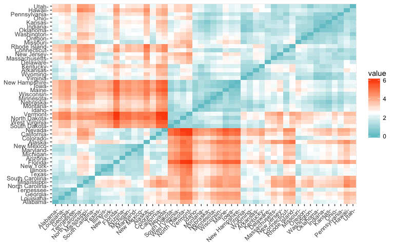
Within R it is simple to compute and visualize the distance matrix using the functions get_dist and fviz_dist from the factoextra R package. This starts to illustrate which states have large dissimilarities (red) versus those that appear to be fairly similar (teal).
get_dist: for computing a distance matrix between the rows of a data matrix. The default distance computed is the Euclidean; however, get_dist also supports distanced described in equations 2-5 above plus others.fviz_dist: for visualizing a distance matrixdistance <- get_dist(df)
fviz_dist(distance, gradient = list(low = "#00AFBB", mid = "white", high = "#FC4E07"))
K-means clustering is the most commonly used unsupervised machine learning algorithm for partitioning a given data set into a set of k groups (i.e. k clusters), where k represents the number of groups pre-specified by the analyst. It classifies objects in multiple groups (i.e., clusters), such that objects within the same cluster are as similar as possible (i.e., high intra-class similarity), whereas objects from different clusters are as dissimilar as possible (i.e., low inter-class similarity). In k-means clustering, each cluster is represented by its center (i.e, centroid) which corresponds to the mean of points assigned to the cluster.
The basic idea behind k-means clustering consists of defining clusters so that the total intra-cluster variation (known as total within-cluster variation) is minimized. There are several k-means algorithms available. The standard algorithm is the Hartigan-Wong algorithm (1979), which defines the total within-cluster variation as the sum of squared distances Euclidean distances between items and the corresponding centroid:
where:
Each observation () is assigned to a given cluster such that the sum of squares (SS) distance of the observation to their assigned cluster centers () is minimized.
We define the total within-cluster variation as follows:
The total within-cluster sum of square measures the compactness (i.e goodness) of the clustering and we want it to be as small as possible.
The first step when using k-means clustering is to indicate the number of clusters (k) that will be generated in the final solution. The algorithm starts by randomly selecting k objects from the data set to serve as the initial centers for the clusters. The selected objects are also known as cluster means or centroids. Next, each of the remaining objects is assigned to it’s closest centroid, where closest is defined using the Euclidean distance (Eq. 1) between the object and the cluster mean. This step is called “cluster assignment step”. After the assignment step, the algorithm computes the new mean value of each cluster. The term cluster “centroid update” is used to design this step. Now that the centers have been recalculated, every observation is checked again to see if it might be closer to a different cluster. All the objects are reassigned again using the updated cluster means. The cluster assignment and centroid update steps are iteratively repeated until the cluster assignments stop changing (i.e until convergence is achieved). That is, the clusters formed in the current iteration are the same as those obtained in the previous iteration.
K-means algorithm can be summarized as follows:
We can compute k-means in R with the kmeans function. Here will group the data into two clusters (centers = 2). The kmeans function also has an nstart option that attempts multiple initial configurations and reports on the best one. For example, adding nstart = 25 will generate 25 initial configurations. This approach is often recommended.
k2 <- kmeans(df, centers = 2, nstart = 25)
str(k2)
## List of 9
##  $ cluster     : Named int [1:50] 1 1 1 2 1 1 2 2 1 1 ...
##   ..- attr(*, "names")= chr [1:50] "Alabama" "Alaska" "Arizona" "Arkansas" ...
##  $ centers     : num [1:2, 1:4] 1.005 -0.67 1.014 -0.676 0.198 ...
##   ..- attr(*, "dimnames")=List of 2
##   .. ..$ : chr [1:2] "1" "2"
##   .. ..$ : chr [1:4] "Murder" "Assault" "UrbanPop" "Rape"
##  $ totss       : num 196
##  $ withinss    : num [1:2] 46.7 56.1
##  $ tot.withinss: num 103
##  $ betweenss   : num 93.1
##  $ size        : int [1:2] 20 30
##  $ iter        : int 1
##  $ ifault      : int 0
##  - attr(*, "class")= chr "kmeans"
The output of kmeans is a list with several bits of information. The most important being:
cluster: A vector of integers (from 1:k) indicating the cluster to which each point is allocated.centers: A matrix of cluster centers.totss: The total sum of squares.withinss: Vector of within-cluster sum of squares, one component per cluster.tot.withinss: Total within-cluster sum of squares, i.e. sum(withinss).betweenss: The between-cluster sum of squares, i.e. $totss-tot.withinss$.size: The number of points in each cluster.If we print the results we’ll see that our groupings resulted in 2 cluster sizes of 30 and 20. We see the cluster centers (means) for the two groups across the four variables (Murder, Assault, UrbanPop, Rape). We also get the cluster assignment for each observation (i.e. Alabama was assigned to cluster 2, Arkansas was assigned to cluster 1, etc.).
k2
## K-means clustering with 2 clusters of sizes 20, 30
##
## Cluster means:
##      Murder    Assault   UrbanPop       Rape
## 1  1.004934  1.0138274  0.1975853  0.8469650
## 2 -0.669956 -0.6758849 -0.1317235 -0.5646433
##
## Clustering vector:
##        Alabama         Alaska        Arizona       Arkansas     California
##              1              1              1              2              1
##       Colorado    Connecticut       Delaware        Florida        Georgia
##              1              2              2              1              1
##         Hawaii          Idaho       Illinois        Indiana           Iowa
##              2              2              1              2              2
##         Kansas       Kentucky      Louisiana          Maine       Maryland
##              2              2              1              2              1
##  Massachusetts       Michigan      Minnesota    Mississippi       Missouri
##              2              1              2              1              1
##        Montana       Nebraska         Nevada  New Hampshire     New Jersey
##              2              2              1              2              2
##     New Mexico       New York North Carolina   North Dakota           Ohio
##              1              1              1              2              2
##       Oklahoma         Oregon   Pennsylvania   Rhode Island South Carolina
##              2              2              2              2              1
##   South Dakota      Tennessee          Texas           Utah        Vermont
##              2              1              1              2              2
##       Virginia     Washington  West Virginia      Wisconsin        Wyoming
##              2              2              2              2              2
##
## Within cluster sum of squares by cluster:
## [1] 46.74796 56.11445
##  (between_SS / total_SS =  47.5 %)
##
## Available components:
##
## [1] "cluster"      "centers"      "totss"        "withinss"
## [5] "tot.withinss" "betweenss"    "size"         "iter"
## [9] "ifault"
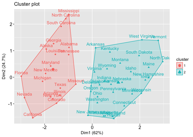
We can also view our results by using fviz_cluster. This provides a nice illustration of the clusters. If there are more than two dimensions (variables) fviz_cluster will perform principal component analysis (PCA) and plot the data points according to the first two principal components that explain the majority of the variance.
fviz_cluster(k2, data = df)
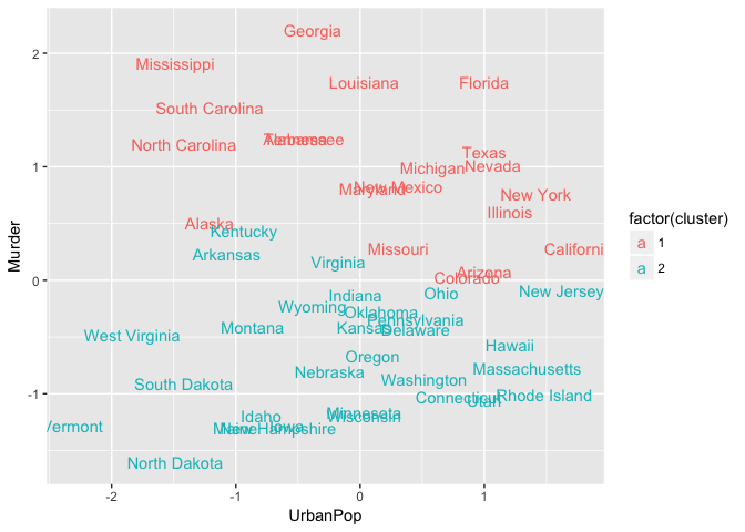
Alternatively, you can use standard pairwise scatter plots to illustrate the clusters compared to the original variables.
df %>%
  as_tibble() %>%
  mutate(cluster = k2$cluster,
         state = row.names(USArrests)) %>%
  ggplot(aes(UrbanPop, Murder, color = factor(cluster), label = state)) +
  geom_text()
Because the number of clusters (k) must be set before we start the algorithm, it is often advantageous to use several different values of k and examine the differences in the results. We can execute the same process for 3, 4, and 5 clusters, and the results are shown in the figure:
k3 <- kmeans(df, centers = 3, nstart = 25)
k4 <- kmeans(df, centers = 4, nstart = 25)
k5 <- kmeans(df, centers = 5, nstart = 25)

# plots to compare
p1 <- fviz_cluster(k2, geom = "point", data = df) + ggtitle("k = 2")
p2 <- fviz_cluster(k3, geom = "point",  data = df) + ggtitle("k = 3")
p3 <- fviz_cluster(k4, geom = "point",  data = df) + ggtitle("k = 4")
p4 <- fviz_cluster(k5, geom = "point",  data = df) + ggtitle("k = 5")

library(gridExtra)
grid.arrange(p1, p2, p3, p4, nrow = 2)
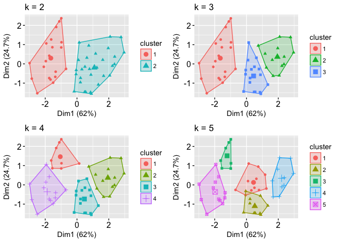
Although this visual assessment tells us where true dilineations occur (or do not occur such as clusters 2 & 4 in the k = 5 graph) between clusters, it does not tell us what the optimal number of clusters is.
As you may recall the analyst specifies the number of clusters to use; preferably the analyst would like to use the optimal number of clusters. To aid the analyst, the following explains the three most popular methods for determining the optimal clusters, which includes:
Recall that, the basic idea behind cluster partitioning methods, such as k-means clustering, is to define clusters such that the total intra-cluster variation (known as total within-cluster variation or total within-cluster sum of square) is minimized:
where is the cluster and is the within-cluster variation. The total within-cluster sum of square (wss) measures the compactness of the clustering and we want it to be as small as possible. Thus, we can use the following algorithm to define the optimal clusters:
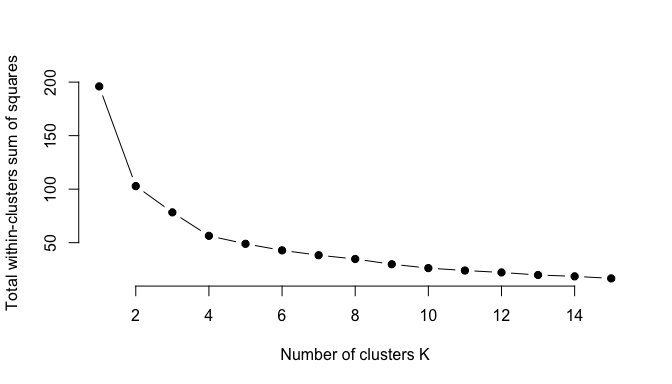
We can implement this in R with the following code. The results suggest that 4 is the optimal number of clusters as it appears to be the bend in the knee (or elbow).
set.seed(123)

# function to compute total within-cluster sum of square
wss <- function(k) {
  kmeans(df, k, nstart = 10 )$tot.withinss
}

# Compute and plot wss for k = 1 to k = 15
k.values <- 1:15

# extract wss for 2-15 clusters
wss_values <- map_dbl(k.values, wss)

plot(k.values, wss_values,
       type="b", pch = 19, frame = FALSE,
       xlab="Number of clusters K",
       ylab="Total within-clusters sum of squares")
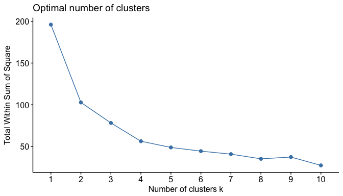
Fortunately, this process to compute the “Elbow method” has been wrapped up in a single function (fviz_nbclust):
set.seed(123)

fviz_nbclust(df, kmeans, method = "wss")
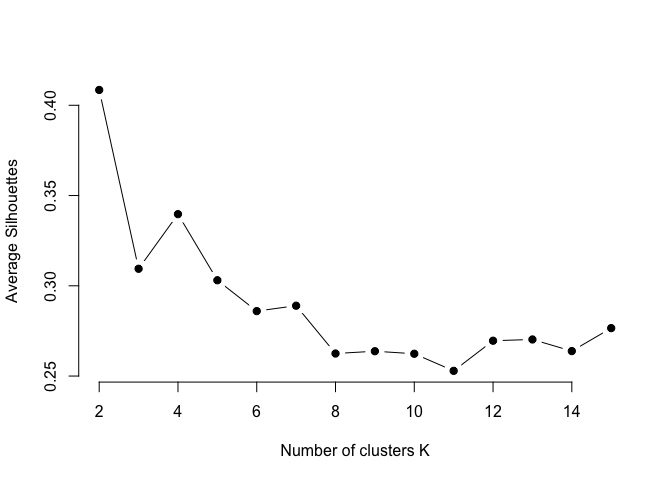
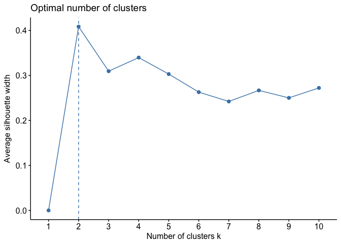
In short, the average silhouette approach measures the quality of a clustering. That is, it determines how well each object lies within its cluster. A high average silhouette width indicates a good clustering. The average silhouette method computes the average silhouette of observations for different values of k. The optimal number of clusters k is the one that maximizes the average silhouette over a range of possible values for k.2
We can use the silhouette function in the cluster package to compuate the average silhouette width. The following code computes this approach for 1-15 clusters. The results show that 2 clusters maximize the average silhouette values with 4 clusters coming in as second optimal number of clusters.
# function to compute average silhouette for k clusters
avg_sil <- function(k) {
  km.res <- kmeans(df, centers = k, nstart = 25)
  ss <- silhouette(km.res$cluster, dist(df))
  mean(ss[, 3])
}

# Compute and plot wss for k = 2 to k = 15
k.values <- 2:15

# extract avg silhouette for 2-15 clusters
avg_sil_values <- map_dbl(k.values, avg_sil)

plot(k.values, avg_sil_values,
       type = "b", pch = 19, frame = FALSE,
       xlab = "Number of clusters K",
       ylab = "Average Silhouettes")
Similar to the elbow method, this process to compute the “average silhoutte method” has been wrapped up in a single function (fviz_nbclust):
fviz_nbclust(df, kmeans, method = "silhouette")
The gap statistic has been published by R. Tibshirani, G. Walther, and T. Hastie (Standford University, 2001). The approach can be applied to any clustering method (i.e. K-means clustering, hierarchical clustering). The gap statistic compares the total intracluster variation for different values of k with their expected values under null reference distribution of the data (i.e. a distribution with no obvious clustering). The reference dataset is generated using Monte Carlo simulations of the sampling process. That is, for each variable () in the data set we compute its range and generate values for the n points uniformly from the interval min to max.
For the observed data and the the reference data, the total intracluster variation is computed using different values of k. The gap statistic for a given k is defined as follow:
Where denotes the expectation under a sample size n from the reference distribution. is defined via bootstrapping (B) by generating B copies of the reference datasets and, by computing the average . The gap statistic measures the deviation of the observed value from its expected value under the null hypothesis. The estimate of the optimal clusters () will be the value that maximizes . This means that the clustering structure is far away from the uniform distribution of points.
In short, the algorithm involves the following steps:
To compute the gap statistic method we can use the clusGap function which provides the gap statistic and standard error for an output.
# compute gap statistic
set.seed(123)
gap_stat <- clusGap(df, FUN = kmeans, nstart = 25,
                    K.max = 10, B = 50)
# Print the result
print(gap_stat, method = "firstmax")
## Clustering Gap statistic ["clusGap"] from call:
## clusGap(x = df, FUNcluster = kmeans, K.max = 10, B = 50, nstart = 25)
## B=50 simulated reference sets, k = 1..10; spaceH0="scaledPCA"
##  --> Number of clusters (method 'firstmax'): 4
##           logW   E.logW       gap     SE.sim
##  [1,] 3.458369 3.638250 0.1798804 0.03653200
##  [2,] 3.135112 3.371452 0.2363409 0.03394132
##  [3,] 2.977727 3.235385 0.2576588 0.03635372
##  [4,] 2.826221 3.120441 0.2942199 0.03615597
##  [5,] 2.738868 3.020288 0.2814197 0.03950085
##  [6,] 2.669860 2.933533 0.2636730 0.03957994
##  [7,] 2.598748 2.855759 0.2570109 0.03809451
##  [8,] 2.531626 2.784000 0.2523744 0.03869283
##  [9,] 2.468162 2.716498 0.2483355 0.03971815
## [10,] 2.394884 2.652241 0.2573567 0.04104674
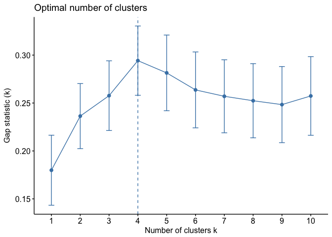
We can visualize the results with fviz_gap_stat which suggests four clusters as the optimal number of clusters.
fviz_gap_stat(gap_stat)
In addition to these commonly used approaches, the NbClust package, published by Charrad et al., 2014, provides 30 indices for determining the relevant number of clusters and proposes to users the best clustering scheme from the different results obtained by varying all combinations of number of clusters, distance measures, and clustering methods.
With most of these approaches suggesting 4 as the number of optimal clusters, we can perform the final analysis and extract the results using 4 clusters.
# Compute k-means clustering with k = 4
set.seed(123)
final <- kmeans(df, 4, nstart = 25)
print(final)
## K-means clustering with 4 clusters of sizes 13, 16, 13, 8
##
## Cluster means:
##       Murder    Assault   UrbanPop        Rape
## 1 -0.9615407 -1.1066010 -0.9301069 -0.96676331
## 2 -0.4894375 -0.3826001  0.5758298 -0.26165379
## 3  0.6950701  1.0394414  0.7226370  1.27693964
## 4  1.4118898  0.8743346 -0.8145211  0.01927104
##
## Clustering vector:
##        Alabama         Alaska        Arizona       Arkansas     California
##              4              3              3              4              3
##       Colorado    Connecticut       Delaware        Florida        Georgia
##              3              2              2              3              4
##         Hawaii          Idaho       Illinois        Indiana           Iowa
##              2              1              3              2              1
##         Kansas       Kentucky      Louisiana          Maine       Maryland
##              2              1              4              1              3
##  Massachusetts       Michigan      Minnesota    Mississippi       Missouri
##              2              3              1              4              3
##        Montana       Nebraska         Nevada  New Hampshire     New Jersey
##              1              1              3              1              2
##     New Mexico       New York North Carolina   North Dakota           Ohio
##              3              3              4              1              2
##       Oklahoma         Oregon   Pennsylvania   Rhode Island South Carolina
##              2              2              2              2              4
##   South Dakota      Tennessee          Texas           Utah        Vermont
##              1              4              3              2              1
##       Virginia     Washington  West Virginia      Wisconsin        Wyoming
##              2              2              1              1              2
##
## Within cluster sum of squares by cluster:
## [1] 11.952463 16.212213 19.922437  8.316061
##  (between_SS / total_SS =  71.2 %)
##
## Available components:
##
## [1] "cluster"      "centers"      "totss"        "withinss"
## [5] "tot.withinss" "betweenss"    "size"         "iter"
## [9] "ifault"
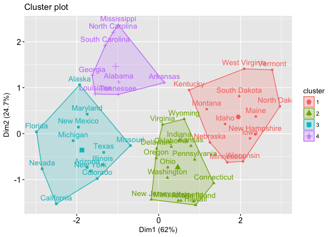
We can visualize the results using fviz_cluster:
fviz_cluster(final, data = df)
And we can extract the clusters and add to our initial data to do some descriptive statistics at the cluster level:
USArrests %>%
  mutate(Cluster = final$cluster) %>%
  group_by(Cluster) %>%
  summarise_all("mean")
## # A tibble: 4 × 5
##   Cluster   Murder   Assault UrbanPop     Rape
##     <int>    <dbl>     <dbl>    <dbl>    <dbl>
## 1       1  3.60000  78.53846 52.07692 12.17692
## 2       2  5.65625 138.87500 73.87500 18.78125
## 3       3 10.81538 257.38462 76.00000 33.19231
## 4       4 13.93750 243.62500 53.75000 21.41250
K-means clustering is a very simple and fast algorithm. Furthermore, it can efficiently deal with very large data sets. However, there are some weaknesses of the k-means approach.
One potential disadvantage of K-means clustering is that it requires us to pre-specify the number of clusters. Hierarchical clustering is an alternative approach which does not require that we commit to a particular choice of clusters. Hierarchical clustering has an added advantage over K-means clustering in that it results in an attractive tree-based representation of the observations, called a dendrogram. A future tutorial will illustrate the hierarchical clustering approach.
An additional disadvantage of K-means is that it’s sensitive to outliers and different results can occur if you change the ordering of your data. The Partitioning Around Medoids (PAM) clustering approach is less sensititive to outliers and provides a robust alternative to k-means to deal with these situations. A future tutorial will illustrate the PAM clustering approach.
For now, you can learn more about clustering methods with:
Standardization makes the four distance measure methods - Euclidean, Manhattan, Correlation and Eisen - more similar than they would be with non-transformed data. ↩