![]() Follow me on twitter @bradleyboehmke
Follow me on twitter @bradleyboehmke
![]() Follow me on twitter @bradleyboehmke
Follow me on twitter @bradleyboehmke
 Logistic regression (aka logit regression or logit model) was developed by statistician David Cox in 1958 and is a regression model where the response variable Y is categorical. Logistic regression allows us to estimate the probability of a categorical response based on one or more predictor variables (X). It allows one to say that the presence of a predictor increases (or decreases) the probability of a given outcome by a specific percentage. This tutorial covers the case when Y is binary — that is, where it can take only two values, “0” and “1”, which represent outcomes such as pass/fail, win/lose, alive/dead or healthy/sick. Cases where the dependent variable has more than two outcome categories may be analysed with multinomial logistic regression, or, if the multiple categories are ordered, in ordinal logistic regression. However, discriminant analysis has become a popular method for multi-class classification so our next tutorial will focus on that technique for those instances.
This tutorial serves as an introduction to logistic regression and covers1:
This tutorial primarily leverages the Default data provided by the ISLR package. This is a simulated data set containing information on ten thousand customers such as whether the customer defaulted, is a student, the average balance carried by the customer and the income of the customer. We’ll also use a few packages that provide data manipulation, visualization, pipeline modeling functions, and model output tidying functions.
# Packages
library(tidyverse)  # data manipulation and visualization
library(modelr)     # provides easy pipeline modeling functions
library(broom)      # helps to tidy up model outputs

# Load data
(default <- as_tibble(ISLR::Default))
## # A tibble: 10,000 × 4
##    default student   balance    income
##     <fctr>  <fctr>     <dbl>     <dbl>
## 1       No      No  729.5265 44361.625
## 2       No     Yes  817.1804 12106.135
## 3       No      No 1073.5492 31767.139
## 4       No      No  529.2506 35704.494
## 5       No      No  785.6559 38463.496
## 6       No     Yes  919.5885  7491.559
## 7       No      No  825.5133 24905.227
## 8       No     Yes  808.6675 17600.451
## 9       No      No 1161.0579 37468.529
## 10      No      No    0.0000 29275.268
## # ... with 9,990 more rows
Linear regression is not appropriate in the case of a qualitative response. Why not? Suppose that we are trying to predict the medical condition of a patient in the emergency room on the basis of her symptoms. In this simplified example, there are three possible diagnoses: stroke, drug overdose, and epileptic seizure. We could consider encoding these values as a quantitative response variable, Y , as follows:
Using this coding, least squares could be used to fit a linear regression model to predict Y on the basis of a set of predictors . Unfortunately, this coding implies an ordering on the outcomes, putting drug overdose in between stroke and epileptic seizure, and insisting that the difference between stroke and drug overdose is the same as the difference between drug overdose and epileptic seizure. In practice there is no particular reason that this needs to be the case. For instance, one could choose an equally reasonable coding,
which would imply a totally different relationship among the three conditions. Each of these codings would produce fundamentally different linear models that would ultimately lead to different sets of predictions on test observations.
More relevant to our data, if we are trying to classify a customer as a high- vs. low-risk defaulter based on their balance we could use linear regression; however, the left figure below illustrates how linear regression would predict the probability of defaulting. Unfortunately, for balances close to zero we predict a negative probability of defaulting; if we were to predict for very large balances, we would get values bigger than 1. These predictions are not sensible, since of course the true probability of defaulting, regardless of credit card balance, must fall between 0 and 1.
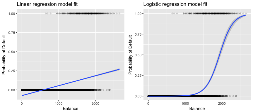
To avoid this problem, we must model p(X) using a function that gives outputs between 0 and 1 for all values of X. Many functions meet this description. In logistic regression, we use the logistic function, which is defined in Eq. 1 and illustrated in the right figure above.
As in the regression tutorial, we’ll split our data into a training (60%) and testing (40%) data sets so we can assess how well our model performs on an out-of-sample data set.
set.seed(123)
sample <- sample(c(TRUE, FALSE), nrow(default), replace = T, prob = c(0.6,0.4))
train <- default[sample, ]
test <- default[!sample, ]
We will fit a logistic regression model in order to predict the probability of a customer defaulting based on the average balance carried by the customer. The glm function fits generalized linear models, a class of models that includes logistic regression. The syntax of the glm function is similar to that of lm, except that we must pass the argument family = binomial in order to tell R to run a logistic regression rather than some other type of generalized linear model.
model1 <- glm(default ~ balance, family = "binomial", data = train)
In the background the glm, uses maximum likelihood to fit the model. The basic intuition behind using maximum likelihood to fit a logistic regression model is as follows: we seek estimates for and such that the predicted probability of default for each individual, using Eq. 1, corresponds as closely as possible to the individual’s observed default status. In other words, we try to find and such that plugging these estimates into the model for p(X), given in Eq. 1, yields a number close to one for all individuals who defaulted, and a number close to zero for all individuals who did not. This intuition can be formalized using a mathematical equation called a likelihood function:
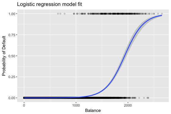
The estimates and are chosen to maximize this likelihood function. Maximum likelihood is a very general approach that is used to fit many of the non-linear models that we will examine in future tutorials. What results is a an S-shaped probability curve illustrated below (note that to plot the logistic regression fit line we need to convert our response variable to a [0,1] binary coded variable).
default %>%
  mutate(prob = ifelse(default == "Yes", 1, 0)) %>%
  ggplot(aes(balance, prob)) +
  geom_point(alpha = .15) +
  geom_smooth(method = "glm", method.args = list(family = "binomial")) +
  ggtitle("Logistic regression model fit") +
  xlab("Balance") +
  ylab("Probability of Default")
Similar to linear regression we can assess the model using summary or glance. Note that the coefficient output format is similar to what we saw in linear regression; however, the goodness-of-fit details at the bottom of summary differ. We’ll get into this more later but just note that you see the word deviance. Deviance is analogous to the sum of squares calculations in linear regression and is a measure of the lack of fit to the data in a logistic regression model. The null deviance represents the difference between a model with only the intercept (which means “no predictors”) and a saturated model (a model with a theoretically perfect fit). The goal is for the model deviance (noted as Residual deviance) to be lower; smaller values indicate better fit. In this respect, the null model provides a baseline upon which to compare predictor models.
summary(model1)
##
## Call:
## glm(formula = default ~ balance, family = "binomial", data = train)
##
## Deviance Residuals:
##     Min       1Q   Median       3Q      Max
## -2.2905  -0.1395  -0.0528  -0.0189   3.3346
##
## Coefficients:
##               Estimate Std. Error z value Pr(>|z|)
## (Intercept) -1.101e+01  4.887e-01  -22.52   <2e-16 ***
## balance      5.669e-03  2.949e-04   19.22   <2e-16 ***
## ---
## Signif. codes:  0 '***' 0.001 '**' 0.01 '*' 0.05 '.' 0.1 ' ' 1
##
## (Dispersion parameter for binomial family taken to be 1)
##
##     Null deviance: 1723.03  on 6046  degrees of freedom
## Residual deviance:  908.69  on 6045  degrees of freedom
## AIC: 912.69
##
## Number of Fisher Scoring iterations: 8
The below table shows the coefficient estimates and related information that result from fitting a logistic regression model in order to predict the probability of default = Yes using balance. Bear in mind that the coefficient estimates from logistic regression characterize the relationship between the predictor and response variable on a log-odds scale (see Ch. 3 of ISLR1 for more details). Thus, we see that ; this indicates that an increase in balance is associated with an increase in the probability of default. To be precise, a one-unit increase in balance is associated with an increase in the log odds of default by 0.0057 units.
tidy(model1)
##          term      estimate   std.error statistic       p.value
## 1 (Intercept) -11.006277528 0.488739437 -22.51972 2.660162e-112
## 2     balance   0.005668817 0.000294946  19.21985  2.525157e-82
We can further interpret the balance coefficient as - for every one dollar increase in monthly balance carried, the odds of the customer defaulting increases by a factor of 1.0057.
exp(coef(model1))
##  (Intercept)      balance
## 1.659718e-05 1.005685e+00
Many aspects of the coefficient output are similar to those discussed in the linear regression output. For example, we can measure the confidence intervals and accuracy of the coefficient estimates by computing their standard errors. For instance, has a p-value < 2e-16 suggesting a statistically significant relationship between balance carried and the probability of defaulting. We can also use the standard errors to get confidence intervals as we did in the linear regression tutorial:
confint(model1)
##                     2.5 %        97.5 %
## (Intercept) -12.007610373 -10.089360652
## balance       0.005111835   0.006269411
Once the coefficients have been estimated, it is a simple matter to compute the probability of default for any given credit card balance. Mathematically, using the coefficient estimates from our model we predict that the default probability for an individual with a balance of $1,000 is less than 0.5%
We can predict the probability of defaulting in R using the predict function (be sure to include type = "response"). Here we compare the probability of defaulting based on balances of $1000 and $2000. As you can see as the balance moves from $1000 to $2000 the probability of defaulting increases signficantly, from 0.5% to 58%!
predict(model1, data.frame(balance = c(1000, 2000)), type = "response")
##           1           2
## 0.004785057 0.582089269
One can also use qualitative predictors with the logistic regression model. As an example, we can fit a model that uses the student variable.
model2 <- glm(default ~ student, family = "binomial", data = train)

tidy(model2)
##          term   estimate  std.error statistic     p.value
## 1 (Intercept) -3.5534091 0.09336545 -38.05914 0.000000000
## 2  studentYes  0.4413379 0.14927208   2.95660 0.003110511
The coefficient associated with student = Yes is positive, and the associated p-value is statistically significant. This indicates that students tend to have higher default probabilities than non-students. In fact, this model suggests that a student has nearly twice the odds of defaulting than non-students. However, in the next section we’ll see why.
predict(model2, data.frame(student = factor(c("Yes", "No"))), type = "response")
##          1          2
## 0.04261206 0.02783019
We can also extend our model as seen in Eq. 1 so that we can predict a binary response using multiple predictors where are p predictors:
Let’s go ahead and fit a model that predicts the probability of default based on the balance, income (in thousands of dollars), and student status variables. There is a surprising result here. The p-values associated with balance and student=Yes status are very small, indicating that each of these variables is associated with the probability of defaulting. However, the coefficient for the student variable is negative, indicating that students are less likely to default than non-students. In contrast, the coefficient for the student variable in model 2, where we predicted the probability of default based only on student status, indicated that students have a greater probability of defaulting. What gives?
model3 <- glm(default ~ balance + income + student, family = "binomial", data = train)
tidy(model3)
##          term      estimate    std.error   statistic      p.value
## 1 (Intercept) -1.090704e+01 6.480739e-01 -16.8299277 1.472817e-63
## 2     balance  5.907134e-03 3.102425e-04  19.0403764 7.895817e-81
## 3      income -5.012701e-06 1.078617e-05  -0.4647343 6.421217e-01
## 4  studentYes -8.094789e-01 3.133150e-01  -2.5835947 9.777661e-03
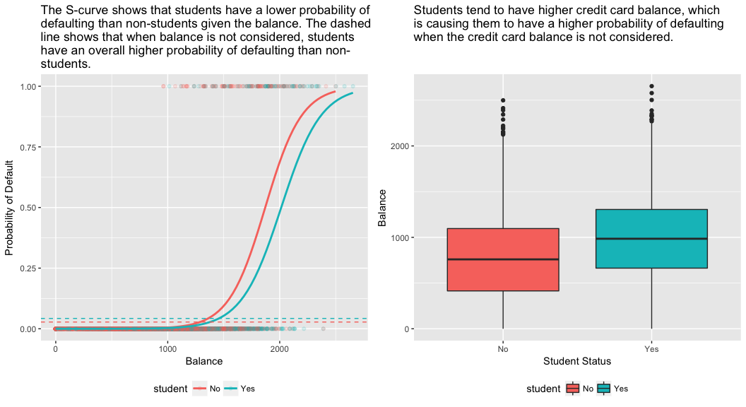
The right-hand panel of the figure below provides an explanation for this discrepancy. The variables student and balance are correlated. Students tend to hold higher levels of debt, which is in turn associated with higher probability of default. In other words, students are more likely to have large credit card balances, which, as we know from the left-hand panel of the below figure, tend to be associated with high default rates. Thus, even though an individual student with a given credit card balance will tend to have a lower probability of default than a non-student with the same credit card balance, the fact that students on the whole tend to have higher credit card balances means that overall, students tend to default at a higher rate than non-students. This is an important distinction for a credit card company that is trying to determine to whom they should offer credit. A student is riskier than a non-student if no information about the student’s credit card balance is available. However, that student is less risky than a non-student with the same credit card balance!
This simple example illustrates the dangers and subtleties associated with performing regressions involving only a single predictor when other predictors may also be relevant. The results obtained using one predictor may be quite different from those obtained using multiple predictors, especially when there is correlation among the predictors. This phenomenon is known as confounding.
In the case of multiple predictor variables sometimes we want to understand which variable is the most influential in predicting the response (Y) variable. We can do this with varImp from the caret package. Here, we see that balance is the most important by a large margin whereas student status is less important followed by income (which was found to be insignificant anyways (p = .64)).
caret::varImp(model3)
##               Overall
## balance    19.0403764
## income      0.4647343
## studentYes  2.5835947
As before, we can easily make predictions with this model. For example, a student with a credit card balance of $1,500 and an income of $40,000 has an estimated probability of default of
A non-student with the same balance and income has an estimated probability of default of
new.df <- tibble(balance = 1500, income = 40, student = c("Yes", "No"))
predict(model3, new.df, type = "response")
##          1          2
## 0.05437124 0.11440288
Thus, we see that for the given balance and income (although income is insignificant) a student has about half the probability of defaulting than a non-student.
So far three logistic regression models have been built and the coefficients have been examined. However, some critical questions remain. Are the models any good? How well does the model fit the data? And how accurate are the predictions on an out-of-sample data set?
In the linear regression tutorial we saw how the F-statistic, and adjusted , and residual diagnostics inform us of how good the model fits the data. Here, we’ll look at a few ways to assess the goodness-of-fit for our logit models.
First, we can use a Likelihood Ratio Test to assess if our models are improving the fit. Adding predictor variables to a model will almost always improve the model fit (i.e. increase the log likelihood and reduce the model deviance compared to the null deviance), but it is necessary to test whether the observed difference in model fit is statistically significant. We can use anova to perform this test. The results indicate that, compared to model1, model3 reduces the residual deviance by over 13 (remember, a goal of logistic regression is to find a model that minimizes deviance residuals). More imporantly, this improvement is statisticallly significant at p = 0.001. This suggests that model3 does provide an improved model fit.
anova(model1, model3, test = "Chisq")
## Analysis of Deviance Table
##
## Model 1: default ~ balance
## Model 2: default ~ balance + income + student
##   Resid. Df Resid. Dev Df Deviance Pr(>Chi)
## 1      6045     908.69
## 2      6043     895.02  2   13.668 0.001076 **
## ---
## Signif. codes:  0 '***' 0.001 '**' 0.01 '*' 0.05 '.' 0.1 ' ' 1
Unlike linear regression with ordinary least squares estimation, there is no statistic which explains the proportion of variance in the dependent variable that is explained by the predictors. However, there are a number of pseudo metrics that could be of value. Most notable is McFadden’s , which is defined as
where is the log likelihood value for the fitted model and is the log likelihood for the null model with only an intercept as a predictor. The measure ranges from 0 to just under 1, with values closer to zero indicating that the model has no predictive power. However, unlike in linear regression, models rarely achieve a high McFadden . In fact, in McFadden’s own words models with a McFadden pseudo represents a very good fit. We can assess McFadden’s pseudo values for our models with:
list(model1 = pscl::pR2(model1)["McFadden"],
     model2 = pscl::pR2(model2)["McFadden"],
     model3 = pscl::pR2(model3)["McFadden"])
## $model1
##  McFadden
## 0.4726215
##
## $model2
##    McFadden
## 0.004898314
##
## $model3
##  McFadden
## 0.4805543
We see that model 2 has a very low value corroborating its poor fit. However, models 1 and 3 are much higher suggesting they explain a fair amount of variance in the default data. Furthermore, we see that model 3 only improves the ever so slightly.
Keep in mind that logistic regression does not assume the residuals are normally distributed nor that the variance is constant. However, the deviance residual is useful for determining if individual points are not well fit by the model. Here we can fit the standardized deviance residuals to see how many exceed 3 standard deviations. First we extract several useful bits of model results with augment and then proceed to plot.
model1_data <- augment(model1) %>%
  mutate(index = 1:n())

ggplot(model1_data, aes(index, .std.resid, color = default)) +
  geom_point(alpha = .5) +
  geom_ref_line(h = 3)
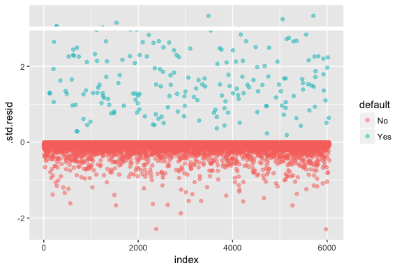
Those standardized residuals that exceed 3 represent possible outliers and may deserve closer attention. We can filter for these residuals to get a closer look. We see that all these observations represent customers who defaulted with budgets that are much lower than the normal defaulters.
model1_data %>%
  filter(abs(.std.resid) > 3)
##   default   balance   .fitted   .se.fit   .resid         .hat    .sigma    .cooksd .std.resid index
## 1     Yes 1118.7010 -4.664566 0.1752745 3.057432 0.0002841609 0.3857438 0.01508609   3.057867   271
## 2     Yes 1119.0972 -4.662320 0.1751742 3.056704 0.0002844621 0.3857448 0.01506820   3.057139   272
## 3     Yes 1135.0473 -4.571902 0.1711544 3.027272 0.0002967274 0.3857832 0.01435943   3.027721  1253
## 4     Yes 1066.8841 -4.958307 0.1885550 3.151288 0.0002463229 0.3856189 0.01754100   3.151676  1542
## 5     Yes  961.4889 -5.555773 0.2163846 3.334556 0.0001796165 0.3853639 0.02324417   3.334855  3488
## 6     Yes 1143.6805 -4.522962 0.1689933 3.011233 0.0003034789 0.3858039 0.01398491   3.011690  4142
## 7     Yes 1013.2169 -5.262537 0.2026075 3.245830 0.0002105772 0.3854892 0.02032614   3.246172  5058
## 8     Yes  961.7327 -5.554391 0.2163192 3.334143 0.0001797543 0.3853645 0.02322988   3.334443  5709
Similar to linear regression we can also identify influential observations with Cook’s distance values. Here we identify the top 5 largest values.
plot(model1, which = 4, id.n = 5)
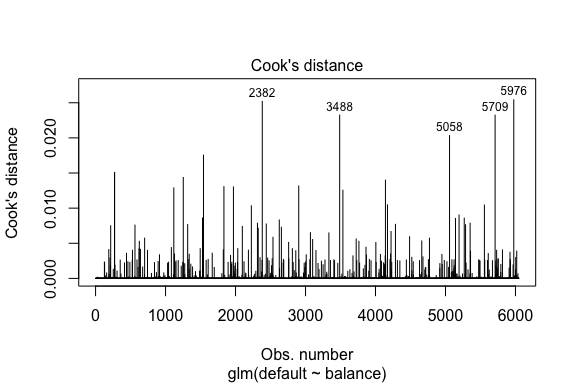
And we can investigate these further as well. Here we see that the top five influential points include:
This means if we were to remove these observations (not recommended), the shape, location, and confidence interval of our logistic regression S-curve would likely shift.
model1_data %>%
  top_n(5, .cooksd)
##   default   balance   .fitted   .se.fit    .resid         .hat    .sigma    .cooksd .std.resid index
## 1      No 2388.1740  2.531843 0.2413764 -2.284011 0.0039757771 0.3866249 0.02520100  -2.288565  2382
## 2     Yes  961.4889 -5.555773 0.2163846  3.334556 0.0001796165 0.3853639 0.02324417   3.334855  3488
## 3     Yes 1013.2169 -5.262537 0.2026075  3.245830 0.0002105772 0.3854892 0.02032614   3.246172  5058
## 4     Yes  961.7327 -5.554391 0.2163192  3.334143 0.0001797543 0.3853645 0.02322988   3.334443  5709
## 5      No 2391.0077  2.547907 0.2421522 -2.290521 0.0039468742 0.3866185 0.02542145  -2.295054  5976
When developing models for prediction, the most critical metric is regarding how well the model does in predicting the target variable on out-of-sample observations. First, we need to use the estimated models to predict values on our training data set (train). When using predict be sure to include type = response so that the prediction returns the probability of default.
test.predicted.m1 <- predict(model1, newdata = test, type = "response")
test.predicted.m2 <- predict(model2, newdata = test, type = "response")
test.predicted.m3 <- predict(model3, newdata = test, type = "response")
Now we can compare the predicted target variable versus the observed values for each model and see which performs the best. We can start by using the confusion matrix, which is a table that describes the classification performance for each model on the test data. Each quadrant of the table has an important meaning. In this case the “No” and “Yes” in the rows represent whether customers defaulted or not. The “FALSE” and “TRUE” in the columns represent whether we predicted customers to default or not.
The results show that model1 and model3 are very similar. 96% of the predicted observations are true negatives and about 1% are true positives. Both models have a type II error of less than 3% in which the model predicts the customer will not default but they actually did. And both models have a type I error of less than 1% in which the models predicts the customer will default but they never did. model2 results are notably different; this model accurately predicts the non-defaulters (a result of 97% of the data being non-defaulters) but never actually predicts those customers that default!
list(
  model1 = table(test$default, test.predicted.m1 > 0.5) %>% prop.table() %>% round(3),
  model2 = table(test$default, test.predicted.m2 > 0.5) %>% prop.table() %>% round(3),
  model3 = table(test$default, test.predicted.m3 > 0.5) %>% prop.table() %>% round(3)
)
## $model1
##
##       FALSE  TRUE
##   No  0.962 0.003
##   Yes 0.025 0.010
##
## $model2
##
##       FALSE
##   No  0.965
##   Yes 0.035
##
## $model3
##
##       FALSE  TRUE
##   No  0.963 0.003
##   Yes 0.026 0.009
We also want to understand the missclassification (aka error) rates (or we could flip this for the accuracy rates). We don’t see much improvement between models 1 and 3 and although model 2 has a low error rate don’t forget that it never accurately predicts customers that actually default.
test %>%
  mutate(m1.pred = ifelse(test.predicted.m1 > 0.5, "Yes", "No"),
         m2.pred = ifelse(test.predicted.m2 > 0.5, "Yes", "No"),
         m3.pred = ifelse(test.predicted.m3 > 0.5, "Yes", "No")) %>%
  summarise(m1.error = mean(default != m1.pred),
            m2.error = mean(default != m2.pred),
            m3.error = mean(default != m3.pred))
## # A tibble: 1 × 3
##     m1.error   m2.error   m3.error
##        <dbl>      <dbl>      <dbl>
## 1 0.02782697 0.03491019 0.02807994
We can gain some additional insights by looking at the raw values (not percentages) in our confusion matrix. Lets look at model 1 to illustrate. We see that there are a total of customers that defaulted. Of the total defaults, were not predicted. Alternatively, we could say that only of default occurrences were predicted - this is known as the the precision (also known as sensitivity) of our model. So while the overall error rate is low, the precision rate is also low, which is not good!
table(test$default, test.predicted.m1 > 0.5)
##
##       FALSE TRUE
##   No   3803   12
##   Yes    98   40
With classification models you will also here the terms sensititivy and specificity when characterizing the performance of the model. As mentioned above sensitivity is synonymous to precision. However, the specificity is the percentage of non-defaulters that are correctly identified, here (the accuracy here is largely driven by the fact that 97% of the observations in our data are non-defaulters). The importance between sensititivy and specificity is dependent on context. In this case, a credit card company is likely to be more concerned with sensititivy since they want to reduce their risk. Therefore, they may be more concerned with tuning a model so that their sensititivy/precision is improved.
The receiving operating characteristic (ROC) is a visual measure of classifier performance. Using the proportion of positive data points that are correctly considered as positive and the proportion of negative data points that are mistakenly considered as positive, we generate a graphic that shows the trade off between the rate at which you can correctly predict something with the rate of incorrectly predicting something. Ultimately, we’re concerned about the area under the ROC curve, or AUC. That metric ranges from 0.50 to 1.00, and values above 0.80 indicate that the model does a good job in discriminating between the two categories which comprise our target variable. We can compare the ROC and AUC for model’s 1 and 2, which show a strong difference in performance. We definitely want our ROC plots to look more like model 1’s (left) rather than model 2’s (right)!
library(ROCR)

par(mfrow=c(1, 2))

prediction(test.predicted.m1, test$default) %>%
  performance(measure = "tpr", x.measure = "fpr") %>%
  plot()

prediction(test.predicted.m2, test$default) %>%
  performance(measure = "tpr", x.measure = "fpr") %>%
  plot()
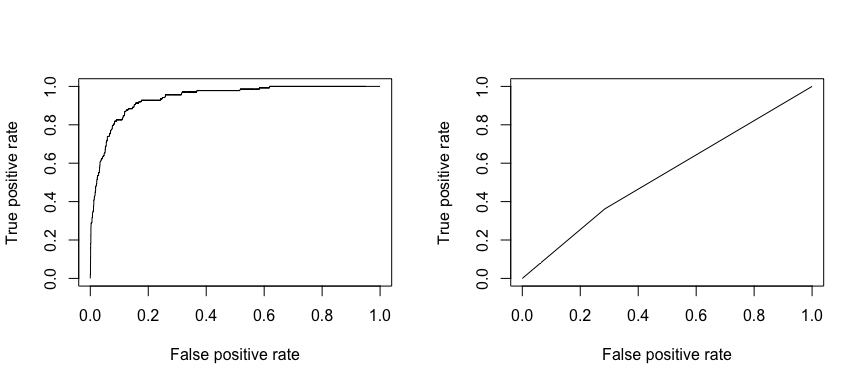
And to compute the AUC numerically we can use the following. Remember, AUC will range from .50 - 1.00. Thus, model 2 is a very poor classifying model while model 1 is a very good classying model.
# model 1 AUC
prediction(test.predicted.m1, test$default) %>%
  performance(measure = "auc") %>%
  .@y.values
## [[1]]
## [1] 0.939932

# model 2 AUC
prediction(test.predicted.m2, test$default) %>%
  performance(measure = "auc") %>%
  .@y.values
## [[1]]
## [1] 0.5386955
We can continue to “tune” our models to improve these classification rates. If you can improve your AUC and ROC curves (which means you are improving the classification accuracy rates) you are creating “lift”, meaning you are lifting the classification accuracy.
This will get you up and running with logistic regression. Keep in mind that there is a lot more you can dig into so the following resources will help you learn more:
This tutorial was built as a supplement to chapter 4, section 3 of An Introduction to Statistical Learning ↩ ↩2