↩

Multivariate Adaptive Regression Splines

Several previous tutorials (i.e. linear regression, logistic regression, regularized regression) discussed algorithms that are intrinsically linear. Many of these models can be adapted to nonlinear patterns in the data by manually adding model terms (i.e. squared terms, interaction effects); however, to do so you must know the specific nature of the nonlinearity a priori. Alternatively, there are numerous algorithms that are inherently nonlinear. When using these models, the exact form of the nonlinearity does not need to be known explicitly or specified prior to model training. Rather, these algorithms will search for, and discover, nonlinearities in the data that help maximize predictive accuracy.

This tutorial discusses multivariate adaptive regression splines (MARS), an algorithm that essentially creates a piecewise linear model which provides an intuitive stepping block into nonlinearity after grasping the concept of linear regression and other intrinsically linear models.

Prerequisites

For this tutorial we will use the following packages:

library(rsample)   # data splitting 
library(ggplot2)   # plotting
library(earth)     # fit MARS models
library(caret)     # automating the tuning process
library(vip)       # variable importance
library(pdp)       # variable relationships

To illustrate various MARS modeling concepts we will use Ames Housing data, which is available via the AmesHousing package.

# Create training (70%) and test (30%) sets for the AmesHousing::make_ames() data.
# Use set.seed for reproducibility

set.seed(123)
ames_split <- initial_split(AmesHousing::make_ames(), prop = .7, strata = "Sale_Price")
ames_train <- training(ames_split)
ames_test  <- testing(ames_split)

The basic idea

Some previous tutorials (i.e. linear regression, logistic regression, regularized regression) have focused on linear models. In those tutorials we illustrated some of the advantages of linear models such as their ease and speed of computation and also the intuitive nature of interpreting their coefficients. However, linear models make a strong assumption about linearity, and this assumption is often a poor one, which can affect predictive accuracy.

We can extend linear models to capture non-linear relationships. Typically, this is done by explicitly including polynomial parameters or step functions. Polynomial regression is a form of regression in which the relationship between the independent variable x and the dependent variable y is modeled as an n $^{th}$ degree polynomial of x. For example, Equation 1 represents a polynomial regression function where y is modeled as a function of x with d degrees. Generally speaking, it is unusual to use d greater than 3 or 4 as the larger d becomes, the easier the function fit becomes overly flexible and oddly shapened…especially near the boundaries of the range of x values.

$y_i = \beta_0 + \beta_1 x_i + \beta_2 x^2_i + \beta_3 x^3_i \dots + \beta_d x^d_i + \epsilon_i, \tag{1}$

An alternative to polynomial regression is step function regression. Whereas polynomial functions impose a global non-linear relationship, step functions break the range of x into bins, and fit a different constant for each bin. This amounts to converting a continuous variable into an ordered categorical variable such that our linear regression function is converted to Equation 2

$y_i = \beta_0 + \beta_1 C_1(x_i) + \beta_2 C_2(x_i) + \beta_3 C_3(x_i) \dots + \beta_d C_d(x_i) + \epsilon_i, \tag{2}$

where $C_1(x)$ represents x values ranging from $c_1 \leq x < c_2$ , $C_2(x)$ represents x values ranging from $c_2 \leq x < c_3$ , $\dots$ , $C_d(x)$ represents x values ranging from $c_{d-1} \leq x < c_d$ . Figure 1 illustrate polynomial and step function fits for Sale_Price as a function of Year_Built in our ames data.

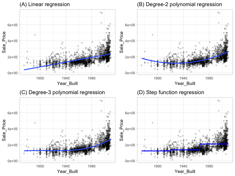
Figure 1: Blue line represents predicted Sale_Price values as a function of Year_Built for alternative approaches to modeling explicit nonlinear regression patterns. (A) Traditional nonlinear regression approach does not capture any nonlinearity unless the predictor or response is transformed (i.e. log transformation). (B) Degree-2 polynomial, (C) Degree-3 polynomial, (D) Step function fitting cutting Year_Built into three categorical levels.

Although useful, the typical implementation of polynomial regression and step functions require the user to explicitly identify and incorporate which variables should have what specific degree of interaction or at what points of a variable x should cut points be made for the step functions. Considering many data sets today can easily contain 50, 100, or more features, this would require an enormous and unncessary time commitment from an analyst to determine these explicit non-linear settings.

Multivariate regression splines

Multivariate adaptive regression splines (MARS) provide a convenient approach to capture the nonlinearity aspect of polynomial regression by assessing cutpoints (knots) similar to step functions. The procedure assesses each data point for each predictor as a knot and creates a linear regression model with the candidate feature(s). For example, consider our simple model of Sale_Price ~ Year_Built. The MARS procedure will first look for the single point across the range of Year_Built values where two different linear relationships between Sale_Price and Year_Built achieve the smallest error. What results is known as a hinge function ( $h(x-a)$ where a is the cutpoint value). For a single knot (Figure 2 (A)), our hinge function is $h(\text{Year_Built}-1968)$ such that our two linear models for Sale_Price are

$\text{Sale_Price} = \begin{cases} 136091.022 & \text{Year_Built} \leq 1968, \\ 136091.022 + 3094.208(\text{Year_Built} - 1968) & \text{Year_Built} > 1968 \end{cases}$

Once the first knot has been found, the search continues for a second knot which is found at 2006 (Figure 2 (B)). This results in three linear models for Sale_Price:

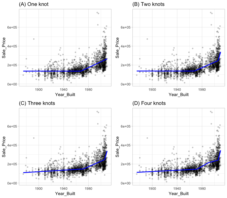
$\text{Sale_Price} = \begin{cases} 136091.022 & \text{Year_Built} \leq 1968, \\ 136091.022 + 2898.424(\text{Year_Built} - 1968) & 1968 < \text{Year_Built} \leq 2006, \\ 136091.022 + 20176.284(\text{Year_Built} - 2006) & \text{Year_Built} > 2006 \end{cases}$

Figure 2: Examples of fitted regression splines of one (A), two (B), three (C), and four (D) knots.

This procedure can continue until many knots are found, producing a highly non-linear pattern. Although including many knots may allow us to fit a really good relationship with our training data, it may not generalize very well to new, unseen data. For example, Figure 3 includes nine knots but this likley will not generalize very well to our test data.

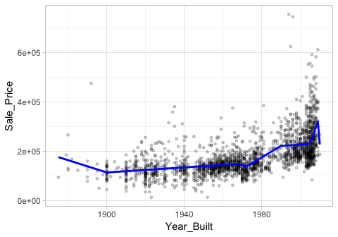
Figure 3: Too many knots may not generalize well to unseen data.

Consequently, once the full set of knots have been created, we can sequentially remove knots that do not contribute significantly to predictive accuracy. This process is known as “pruning” and we can use cross-validation, as we have with the previous models, to find the optimal number of knots.

Fitting a basic MARS model

We can fit a MARS model with the earth package. By default, earth::earth() will assess all potential knots across all supplied features and then will prune to the optimal number of knots based on an expected change in $R^2$ (for the training data) of less than 0.001. This calculation is performed by the Generalized cross-validation procedure (GCV statistic), which is a computational shortcut for linear models that produces an error value that approximates leave-one-out cross-validation (see here for technical details).

Note: The term “MARS” is trademarked and licensed exclusively to Salford Systems http://www.salfordsystems.com. We can use MARS as an abbreviation; however, it cannot be used for competing software solutions. This is why the R package uses the name earth.

The following applies a basic MARS model to our ames data and performs a search for required knots across all features. The results show us the final models GCV statistic, generalized $R^2$ (GRSq), and more.

# Fit a basic MARS model
mars1 <- earth(
  Sale_Price ~ .,  
  data = ames_train   
)

# Print model summary
print(mars1)
## Selected 37 of 45 terms, and 26 of 307 predictors
## Termination condition: RSq changed by less than 0.001 at 45 terms
## Importance: Gr_Liv_Area, Year_Built, Total_Bsmt_SF, ...
## Number of terms at each degree of interaction: 1 36 (additive model)
## GCV 521186626    RSS 995776275391    GRSq 0.9165386    RSq 0.92229

It also shows us that 38 of 41 terms were used from 27 of the 307 original predictors. But what does this mean? If we were to look at all the coefficients, we would see that there are 38 terms in our model (including the intercept). These terms include hinge functions produced from the original 307 predictors (307 predictors because the model automatically dummy encodes our categorical variables). Looking at the first 10 terms in our model, we see that Gr_Liv_Area is included with a knot at 2945 (the coefficient for $h(2945-Gr\_Liv\_Area)$ is -49.85), Year_Built is included with a knot at 2003, etc.

Tip: You can check out all the coefficients with summary(mars1).

summary(mars1) %>% .$coefficients %>% head(10)
##                              Sale_Price
## (Intercept)                301399.98345
## h(2945-Gr_Liv_Area)           -49.84518
## h(Year_Built-2003)           2698.39864
## h(2003-Year_Built)           -357.11319
## h(Total_Bsmt_SF-2171)        -265.30709
## h(2171-Total_Bsmt_SF)         -29.77024
## Overall_QualExcellent       88345.90068
## Overall_QualVery_Excellent 116330.48509
## Overall_QualVery_Good       36646.55568
## h(Bsmt_Unf_SF-278)            -21.15661

The plot method for MARS model objects provide convenient performance and residual plots. Figure 4 illustrates the model selection plot that graphs the GCV $R^2$ (left-hand y-axis and solid black line) based on the number of terms retained in the model (x-axis) which are constructed from a certain number of original predictors (right-hand y-axis). The vertical dashed lined at 37 tells us the optimal number of non-intercept terms retained where marginal increases in GCV $R^2$ are less than 0.001.

plot(mars1, which = 1)

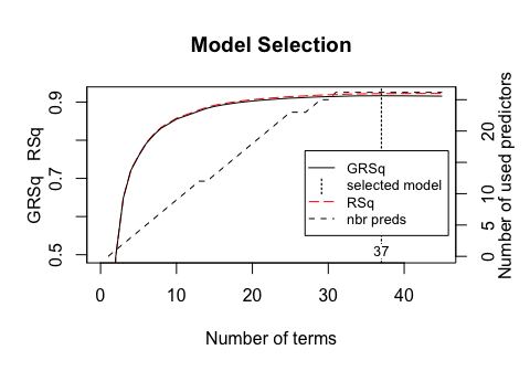
Figure 4: Model summary capturing GCV $R^2$ (left-hand y-axis and solid black line) based on the number of terms retained (x-axis) which is based on the number of predictors used to make those terms (right-hand side y-axis). For this model, 37 non-intercept terms were retained which are based on 26 predictors. Any additional terms retained in the model, over and above these 37, results in less than 0.001 improvement in the GCV $R^2$.

In addition to pruning the number of knots, earth::earth() allows us to also assess potential interactions between different hinge functions. The following illustrates by including a degree = 2 argument. You can see that now our model includes interaction terms between multiple hinge functions (i.e. h(Year_Built-2003)*h(Gr_Liv_Area-2274)) is an interaction effect for those houses built prior to 2003 and have less than 2,274 square feet of living space above ground).

# Fit a basic MARS model
mars2 <- earth(
  Sale_Price ~ .,  
  data = ames_train,
  degree = 2
)

# check out the first 10 coefficient terms
summary(mars2) %>% .$coefficients %>% head(10)
##                                             Sale_Price
## (Intercept)                               242611.63686
## h(Gr_Liv_Area-2945)                          144.39175
## h(2945-Gr_Liv_Area)                          -57.71864
## h(Year_Built-2003)                         10909.70322
## h(2003-Year_Built)                          -780.24246
## h(Year_Built-2003)*h(Gr_Liv_Area-2274)        18.54860
## h(Year_Built-2003)*h(2274-Gr_Liv_Area)       -10.30826
## h(Total_Bsmt_SF-1035)                         62.11901
## h(1035-Total_Bsmt_SF)                        -33.03537
## h(Total_Bsmt_SF-1035)*Kitchen_QualTypical    -32.75942

Tuning

Since there are two tuning parameters associated with our MARS model: the degree of interactions and the number of retained terms, we need to perform a grid search to identify the optimal combination of these hyperparameters that minimize prediction error (the above pruning process was based only on an approximation of cross-validated performance on the training data rather than an actual k-fold cross validation process). As in previous tutorials, we will perform a cross-validated grid search to identify the optimal mix. Here, we set up a search grid that assesses 30 different combinations of interaction effects (degree) and the number of terms to retain (nprune).

# create a tuning grid
hyper_grid <- expand.grid(
  degree = 1:3, 
  nprune = seq(2, 100, length.out = 10) %>% floor()
  )

head(hyper_grid)
##   degree nprune
## 1      1      2
## 2      2      2
## 3      3      2
## 4      1     12
## 5      2     12
## 6      3     12

We can use caret to perform a grid search using 10-fold cross-validation. The model that provides the optimal combination includes second degree interactions and retains 34 terms. The cross-validated RMSE for these models are illustrated in Figure 5 and the optimal model’s cross-validated RMSE is $24,021.68.

Note: This grid search took 5 minutes to complete.

# for reproducibiity
set.seed(123)

# cross validated model
tuned_mars <- train(
  x = subset(ames_train, select = -Sale_Price),
  y = ames_train$Sale_Price,
  method = "earth",
  metric = "RMSE",
  trControl = trainControl(method = "cv", number = 10),
  tuneGrid = hyper_grid
)

# best model
tuned_mars$bestTune
##    nprune degree
## 14     34      2

# plot results
ggplot(tuned_mars)

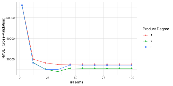
$Figure 5: Cross-validated RMSE for the 30 different hyperparameter combinations in our grid search. The optimal model retains 34 terms and includes up to 2$^{nd}$ degree interactions.$

Figure 5: Cross-validated RMSE for the 30 different hyperparameter combinations in our grid search. The optimal model retains 34 terms and includes up to 2nd degree interactions.

The above grid search helps to focus where we can further refine our model tuning. As a next step, we could perform a grid search that focuses in on a refined grid space for nprune (i.e. comparing 25-40 terms retained). However, for brevity we will leave this as an exercise for the reader.

So how does this compare to some other linear models for the Ames housing data? The following table compares the cross-validated RMSE for our tuned MARS model to a regular multiple regression model along with tuned principal component regression (PCR), partial least squares (PLS), and regularized regression (elastic net) models. By incorporating non-linear relationships and interaction effects, the MARS model provides a substantial improvement over the previous linear models that we have explored.

Note: Notice that we standardize the features for the linear models but we did not for the MARS model. Whereas linear models tend to be sensitive to the scale of the features, MARS models are not.

# multiple regression
set.seed(123)
cv_model1 <- train(
  Sale_Price ~ ., 
  data = ames_train, 
  method = "lm",
  metric = "RMSE",
  trControl = trainControl(method = "cv", number = 10),
  preProcess = c("zv", "center", "scale")
  )

# principal component regression
set.seed(123)
cv_model2 <- train(
  Sale_Price ~ ., 
  data = ames_train, 
  method = "pcr",
  trControl = trainControl(method = "cv", number = 10),
  metric = "RMSE",
  preProcess = c("zv", "center", "scale"),
  tuneLength = 20
  )

# partial least squares regression
set.seed(123)
cv_model3 <- train(
  Sale_Price ~ ., 
  data = ames_train, 
  method = "pls",
  trControl = trainControl(method = "cv", number = 10),
  metric = "RMSE",
  preProcess = c("zv", "center", "scale"),
  tuneLength = 20
  )

# regularized regression
set.seed(123)
cv_model4 <- train(
  Sale_Price ~ ., 
  data = ames_train,
  method = "glmnet",
  trControl = trainControl(method = "cv", number = 10),
  metric = "RMSE",
  preProcess = c("zv", "center", "scale"),
  tuneLength = 10
)

# extract out of sample performance measures
summary(resamples(list(
  Multiple_regression = cv_model1, 
  PCR = cv_model2, 
  PLS = cv_model3,
  Elastic_net = cv_model4,
  MARS = tuned_mars
  )))$statistics$RMSE %>%
  kableExtra::kable() %>%
  kableExtra::kable_styling(bootstrap_options = c("striped", "hover"))

	Min.	1st Qu.	Median	Mean	3rd Qu.	Max.
Multiple_regression	21304.89	24402.89	46474.70	41438.00	53957.79	63246.61
PCR	28213.52	30774.58	36547.70	35769.99	40252.77	44759.98
PLS	22812.20	24196.47	31161.78	31522.47	35383.46	44894.62
Elastic_net	20969.67	24265.17	30590.49	30716.68	34216.06	45241.09
MARS	18439.82	20744.73	23147.04	24021.68	26241.44	31755.20

Feature interpretation

MARS models via earth::earth() include a backwards elimination feature selection routine that looks at reductions in the GCV estimate of error as each predictor is added to the model. This total reduction is used as the variable importance measure (value = "gcv"). Since MARS will automatically include and exclude terms during the pruning process, it essentially performs automated feature selection. If a predictor was never used in any of the MARS basis functions in the final model (after pruning), it has an importance value of zero. This is illustrated in Figure 6 where 27 features have $>0$ importance values while the rest of the features have an importance value of zero since they were not included in the final model. Alternatively, you can also monitor the change in the residual sums of squares (RSS) as terms are added (value = "rss"); however, you will see very little difference between these methods.

# variable importance plots
p1 <- vip(tuned_mars, num_features = 40, bar = FALSE, value = "gcv") + ggtitle("GCV")
p2 <- vip(tuned_mars, num_features = 40, bar = FALSE, value = "rss") + ggtitle("RSS")

gridExtra::grid.arrange(p1, p2, ncol = 2)

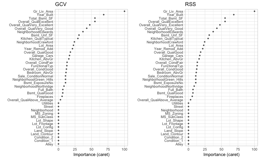
Figure 6: Variable importance based on impact to GCV (left) and RSS (right) values as predictors are added to the model. Both variable importance measures will usually give you very similar results.

Its important to realize that variable importance will only measure the impact of the prediction error as features are included; however, it does not measure the impact for particular hinge functions created for a given feature. For example, in Figure 6 we see that Gr_Liv_Area and Year_Built are the two most influential variables; however, variable importance does not tell us how our model is treating the non-linear patterns for each feature. Also, if we look at the interaction terms our model retained, we see interactions between different hinge functions for Gr_Liv_Area and Year_Built.

coef(tuned_mars$finalModel) %>%
  tidy() %>%
  dplyr::filter(stringr::str_detect(names, "\\*"))
## # A tibble: 16 x 2
##    names                                                   x
##    <chr>                                               <dbl>
##  1 h(Year_Built-2003) * h(Gr_Liv_Area-2274)           18.7  
##  2 h(Year_Built-2003) * h(2274-Gr_Liv_Area)          -10.9  
##  3 h(Total_Bsmt_SF-1035) * Kitchen_QualTypical       -33.1  
##  4 NeighborhoodEdwards * h(Gr_Liv_Area-2945)        -507.   
##  5 h(Lot_Area-4058) * h(3-Garage_Cars)                -0.791
##  6 h(2003-Year_Built) * h(Year_Remod_Add-1974)         7.00 
##  7 Overall_QualExcellent * h(Total_Bsmt_SF-1035)     104.   
##  8 NeighborhoodCrawford * h(2003-Year_Built)         424.   
##  9 h(Lot_Area-4058) * Overall_CondFair                -3.29 
## 10 Overall_QualAbove_Average * h(2003-Year_Built)    136.   
## 11 h(Lot_Area-4058) * Overall_CondGood                 1.35 
## 12 Bsmt_ExposureNo * h(Total_Bsmt_SF-1035)           -22.5  
## 13 NeighborhoodGreen_Hills * h(5-Bedroom_AbvGr)    27362.   
## 14 Overall_QualVery_Good * Bsmt_QualGood          -18641.   
## 15 h(2003-Year_Built) * Sale_ConditionNormal         192.   
## 16 h(Lot_Area-4058) * h(Full_Bath-2)                   1.61

To better understand the relationship between these features and Sale_Price, we can create partial dependence plots (PDPs) for each feature individually and also an interaction PDP. The individual PDPs illustrate that our model found that one knot in each feature provides the best fit. For Gr_Liv_Area, as homes exceed 2,945 square feet, each additional square foot demands a higher marginal increase in sale price than homes with less than 2,945 square feet. Similarly, for homes built after 2003, there is a greater marginal effect on sales price based on the age of the home than for homes built prior to 2003. The interaction plot (far right plot) illustrates the strong effect these two features have when combined.

p1 <- partial(tuned_mars, pred.var = "Gr_Liv_Area", grid.resolution = 10) %>% autoplot()
p2 <- partial(tuned_mars, pred.var = "Year_Built", grid.resolution = 10) %>% autoplot()
p3 <- partial(tuned_mars, pred.var = c("Gr_Liv_Area", "Year_Built"), grid.resolution = 10) %>% 
  plotPartial(levelplot = FALSE, zlab = "yhat", drape = TRUE, colorkey = TRUE, screen = list(z = -20, x = -60))

gridExtra::grid.arrange(p1, p2, p3, ncol = 3)

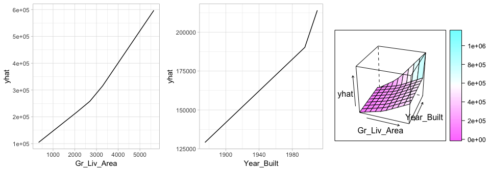
Figure 7: Partial dependence plots to understand the relationship between Sale_Price and the Gr_Liv_Area and Year_Built features. The PDPs tell us that as Gr_Liv_Area increases and for newer homes, Sale_Price increases dramatically.

Final thoughts

MARS provides a great stepping stone into nonlinear modeling and tends to be fairly intuitive due to being closely related to multiple regression techniques. They are also easy to train and tune. This tutorial illustrated how incorporating non-linear relationships via MARS modeling greatly improved predictive accuracy on our Ames housing data. The following summarizes some of the advantages and disadvantages discussed regarding MARS modeling:

Advantages:

Accurate if the local linear relationships are correct.
Quick computation.
Can work well even with large and small data sets.
Provides automated feature selection.
The non-linear relationship between the features and response are fairly intuitive.
Can be used for both regression and classification problems.
Does not require feature standardization.

Disadvantages:

Not accurate if the local linear relationships are incorrect.
Typically not as accurate as more advanced non-linear algorithms (random forests, gradient boosting machines).
The earth package does not incorporate more advanced spline features (i.e. Piecewise cubic models).
Missing values must be pre-processed.

Learning more

This will get you up and running with MARS modeling. Keep in mind that there is a lot more you can dig into so the following resources will help you learn more:

An Introduction to Statistical Learning, Ch. 7
Applied Predictive Modeling, Ch. 7
Elements of Statistical Learning, Ch. 5
Notes on the earth package by Stephen Milborrow

UC Business Analytics R Programming Guide