![]() Follow me on twitter @bradleyboehmke
Follow me on twitter @bradleyboehmke
![]() Follow me on twitter @bradleyboehmke
Follow me on twitter @bradleyboehmke
 Basic regression trees partition a data set into smaller groups and then fit a simple model (constant) for each subgroup. Unfortunately, a single tree model tends to be highly unstable and a poor predictor. However, by bootstrap aggregating (bagging) regression trees, this technique can become quite powerful and effective. Moreover, this provides the fundamental basis of more complex tree-based models such as random forests and gradient boosting machines. This tutorial will get you started with regression trees and bagging.
This tutorial serves as an introduction to the Regression Decision Trees. This tutorial will cover the following material:
This tutorial leverages the following packages. Most of these packages are playing a supporting role while the main emphasis will be on the rpart package.
library(rsample)     # data splitting
library(dplyr)       # data wrangling
library(rpart)       # performing regression trees
library(rpart.plot)  # plotting regression trees
library(ipred)       # bagging
library(caret)       # bagging
To illustrate various regularization concepts we will use the Ames Housing data that has been included in the AmesHousing package.
# Create training (70%) and test (30%) sets for the AmesHousing::make_ames() data.
# Use set.seed for reproducibility

set.seed(123)
ames_split <- initial_split(AmesHousing::make_ames(), prop = .7)
ames_train <- training(ames_split)
ames_test  <- testing(ames_split)
There are many methodologies for constructing regression trees but one of the oldest is known as the classification and regression tree (CART) approach developed by Breiman et al. (1984). This tutorial focuses on the regression part of CART. Basic regression trees partition a data set into smaller subgroups and then fit a simple constant for each observation in the subgroup. The partitioning is achieved by successive binary partitions (aka recursive partitioning) based on the different predictors. The constant to predict is based on the average response values for all observations that fall in that subgroup.
For example, consider we want to predict the miles per gallon a car will average based on cylinders (cyl) and horsepower (hp). All observations go through this tree, are assessed at a particular node, and proceed to the left if the answer is “yes” or proceed to the right if the answer is “no”. So, first, all observations that have 6 or 8 cylinders go to the left branch, all other observations proceed to the right branch. Next, the left branch is further partitioned by horsepower. Those 6 or 8 cylinder observations with horsepower equal to or greater than 192 proceed to the left branch; those with less than 192 hp proceed to the right. These branches lead to terminal nodes or leafs which contain our predicted response value. Basically, all observations (cars in this example) that do not have 6 or 8 cylinders (far right branch) average 27 mpg. All observations that have 6 or 8 cylinders and have more than 192 hp (far left branch) average 13 mpg.
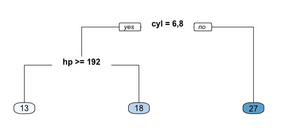
Fig 1. Predicting mpg based on cyl & hp.
This simple example can be generalized to state we have a continuous response variable and two inputs and . The recursive partitioning results in three regions () where the model predicts Y with a constant $c_m$ for region :
However, an important question remains of how to grow a regression tree.
First, its important to realize the partitioning of variables are done in a top-down, greedy fashion. This just means that a partition performed earlier in the tree will not change based on later partitions. But how are these partions made? The model begins with the entire data set, S, and searches every distinct value of every input variable to find the predictor and split value that partitions the data into two regions ( and ) such that the overall sums of squares error are minimized:
Having found the best split, we partition the data into the two resulting regions and repeat the splitting process on each of the two regions. This process is continued until some stopping criterion is reached. What results is, typically, a very deep, complex tree that may produce good predictions on the training set, but is likely to overfit the data, leading to poor performance on unseen data.
For example, using the well-known Boston housing data set, I create three decision trees based on three different samples of the data. You can see that the first few partitions are fairly similar at the top of each tree; however, they tend to differ substantially closer to the terminal nodes. These deeper nodes tend to overfit to specific attributes of the sample data; consequently, slightly different samples will result in highly variable estimate/predicted values in the terminal nodes. By pruning these lower level decision nodes, we can introduce a little bit of bias in our model that help to stabilize predictions and will tend to generalize better to new, unseen data.

Fig 2. Three decision trees based on slightly different samples.
There is often a balance to be achieved in the depth and complexity of the tree to optimize predictive performance on some unseen data. To find this balance, we typically grow a very large tree as defined in the previous section and then prune it back to find an optimal subtree. We find the optimal subtree by using a cost complexity parameter () that penalizes our objective function in Eq. 2 for the number of terminal nodes of the tree (T) as in Eq. 3.
For a given value of , we find the smallest pruned tree that has the lowest penalized error. If you are familiar with regularized regression, you will realize the close association to the lasso norm penalty. As with these regularization methods, smaller penalties tend to produce more complex models, which result in larger trees. Whereas larger penalties result in much smaller trees. Consequently, as a tree grows larger, the reduction in the SSE must be greater than the cost complexity penalty. Typically, we evaluate multiple models across a spectrum of and use cross-validation to identify the optimal and, therefore, the optimal subtree.
There are several advantages to regression trees:
But there are also some significant weaknesses:
We can fit a regression tree using rpart and then visualize it using rpart.plot. The fitting process and the visual output of regression trees and classification trees are very similar. Both use the formula method for expressing the model (similar to lm). However, when fitting a regression tree, we need to set method = "anova". By default, rpart will make an intelligent guess as to what the method value should be based on the data type of your response column, but it’s recommened that you explictly set the method for reproducibility reasons (since the auto-guesser may change in the future).
m1 <- rpart(
  formula = Sale_Price ~ .,
  data    = ames_train,
  method  = "anova"
  )
Once we’ve fit our model we can take a peak at the m1 output. This just explains steps of the splits. For example, we start with 2051 observations at the root node (very beginning) and the first variable we split on (the first variable that optimizes a reduction in SSE) is Overall_Qual. We see that at the first node all observations with Overall_Qual=Very_Poor,Poor,Fair,Below_Average,Average,Above_Average,Good go to the 2nd (2)) branch. The total number of observations that follow this branch (1699), their average sales price (156147.10) and SSE (4.001092e+12) are listed. If you look for the 3rd branch (3)) you will see that 352 observations with Overall_Qual=Very_Good,Excellent,Very_Excellent follow this branch and their average sales prices is 304571.10 and the SEE in this region is 2.874510e+12. Basically, this is telling us the most important variable that has the largest reduction in SEE initially is Overall_Qual with those homes on the upper end of the quality spectrum having almost double the average sales price.
m1
## n= 2051
##
## node), split, n, deviance, yval
##       * denotes terminal node
##
##  1) root 2051 1.329920e+13 181620.20
##    2) Overall_Qual=Very_Poor,Poor,Fair,Below_Average,Average,Above_Average,Good 1699 4.001092e+12 156147.10
##      4) Neighborhood=North_Ames,Old_Town,Edwards,Sawyer,Mitchell,Brookside,Iowa_DOT_and_Rail_Road,South_and_West_of_Iowa_State_University,Meadow_Village,Briardale,Northpark_Villa,Blueste 1000 1.298629e+12 131787.90
##        8) Overall_Qual=Very_Poor,Poor,Fair,Below_Average 195 1.733699e+11  98238.33 *
##        9) Overall_Qual=Average,Above_Average,Good 805 8.526051e+11 139914.80
##         18) First_Flr_SF< 1150.5 553 3.023384e+11 129936.80 *
##         19) First_Flr_SF>=1150.5 252 3.743907e+11 161810.90 *
##      5) Neighborhood=College_Creek,Somerset,Northridge_Heights,Gilbert,Northwest_Ames,Sawyer_West,Crawford,Timberland,Northridge,Stone_Brook,Clear_Creek,Bloomington_Heights,Veenker,Green_Hills 699 1.260199e+12 190995.90
##       10) Gr_Liv_Area< 1477.5 300 2.472611e+11 164045.20 *
##       11) Gr_Liv_Area>=1477.5 399 6.311990e+11 211259.60
##         22) Total_Bsmt_SF< 1004.5 232 1.640427e+11 192946.30 *
##         23) Total_Bsmt_SF>=1004.5 167 2.812570e+11 236700.80 *
##    3) Overall_Qual=Very_Good,Excellent,Very_Excellent 352 2.874510e+12 304571.10
##      6) Overall_Qual=Very_Good 254 8.855113e+11 273369.50
##       12) Gr_Liv_Area< 1959.5 155 3.256677e+11 247662.30 *
##       13) Gr_Liv_Area>=1959.5 99 2.970338e+11 313618.30 *
##      7) Overall_Qual=Excellent,Very_Excellent 98 1.100817e+12 385440.30
##       14) Gr_Liv_Area< 1990 42 7.880164e+10 325358.30 *
##       15) Gr_Liv_Area>=1990 56 7.566917e+11 430501.80
##         30) Neighborhood=College_Creek,Edwards,Timberland,Veenker 8 1.153051e+11 281887.50 *
##         31) Neighborhood=Old_Town,Somerset,Northridge_Heights,Northridge,Stone_Brook 48 4.352486e+11 455270.80
##           62) Total_Bsmt_SF< 1433 12 3.143066e+10 360094.20 *
##           63) Total_Bsmt_SF>=1433 36 2.588806e+11 486996.40 *
We can visualize our model with rpart.plot. rpart.plot has many plotting options, which we’ll leave to the reader to explore. However, in the default print it will show the percentage of data that fall to that node and the average sales price for that branch. One thing you may notice is that this tree contains 11 internal nodes resulting in 12 terminal nodes. Basically, this tree is partitioning on 11 variables to produce its model. However, there are 80 variables in ames_train. So what happened?
rpart.plot(m1)

Behind the scenes rpart is automatically applying a range of cost complexity ( values to prune the tree. To compare the error for each value, rpart performs a 10-fold cross validation so that the error associated with a given value is computed on the hold-out validation data. In this example we find diminishing returns after 12 terminal nodes as illustrated below (y-axis is cross validation error, lower x-axis is cost complexity () value, upper x-axis is the number of terminal nodes (tree size = ). You may also notice the dashed line which goes through the point . Breiman et al. (1984) suggested that in actual practice, its common to instead use the smallest tree within 1 standard deviation of the minimum cross validation error (aka the 1-SE rule). Thus, we could use a tree with 9 terminal nodes and reasonably expect to experience similar results within a small margin of error.
plotcp(m1)

To illustrate the point of selecting a tree with 12 terminal nodes (or 9 if you go by the 1-SE rule), we can force rpart to generate a full tree by using cp = 0 (no penalty results in a fully grown tree). We can see that after 12 terminal nodes, we see diminishing returns in error reduction as the tree grows deeper. Thus, we can signifcantly prune our tree and still achieve minimal expected error.
m2 <- rpart(
    formula = Sale_Price ~ .,
    data    = ames_train,
    method  = "anova",
    control = list(cp = 0, xval = 10)
)

plotcp(m2)
abline(v = 12, lty = "dashed")

So, by default, rpart is performing some automated tuning, with an optimal subtree of 11 splits, 12 terminal nodes, and a cross-validated error of 0.272 (note that this error is equivalent to the PRESS statistic but not the MSE). However, we can perform additional tuning to try improve model performance.
m1$cptable
##            CP nsplit rel error    xerror       xstd
## 1  0.48300624      0 1.0000000 1.0004123 0.05764633
## 2  0.10844747      1 0.5169938 0.5188332 0.02907560
## 3  0.06678458      2 0.4085463 0.4136749 0.02843093
## 4  0.02870391      3 0.3417617 0.3618029 0.02186470
## 5  0.02050153      4 0.3130578 0.3349580 0.02155188
## 6  0.01995037      5 0.2925563 0.3241575 0.02156428
## 7  0.01976132      6 0.2726059 0.3190329 0.02136868
## 8  0.01550003      7 0.2528446 0.3005101 0.02241178
## 9  0.01397824      8 0.2373446 0.2869891 0.02007437
## 10 0.01322455      9 0.2233663 0.2851092 0.02014241
## 11 0.01089820     10 0.2101418 0.2710749 0.02039695
## 12 0.01000000     11 0.1992436 0.2721490 0.02103969
In addition to the cost complexity () parameter, it is also common to tune:
minsplit: the minimum number of data points required to attempt a split before it is forced to create a terminal node. The default is 20. Making this smaller allows for terminal nodes that may contain only a handful of observations to create the predicted value.maxdepth: the maximum number of internal nodes between the root node and the terminal nodes. The default is 30, which is quite liberal and allows for fairly large trees to be built.rpart uses a special control argument where we provide a list of hyperparameter values. For example, if we wanted to assess a model with minsplit = 10 and maxdepth = 12, we could execute the following:
m3 <- rpart(
    formula = Sale_Price ~ .,
    data    = ames_train,
    method  = "anova",
    control = list(minsplit = 10, maxdepth = 12, xval = 10)
)

m3$cptable
##            CP nsplit rel error    xerror       xstd
## 1  0.48300624      0 1.0000000 1.0004637 0.05762992
## 2  0.10844747      1 0.5169938 0.5178889 0.02902537
## 3  0.06678458      2 0.4085463 0.4127568 0.02836546
## 4  0.02870391      3 0.3417617 0.3564832 0.02166543
## 5  0.02050153      4 0.3130578 0.3271474 0.02133529
## 6  0.01995037      5 0.2925563 0.3222644 0.02255183
## 7  0.01976132      6 0.2726059 0.3167303 0.02269857
## 8  0.01550003      7 0.2528446 0.2906408 0.02162499
## 9  0.01397824      8 0.2373446 0.2800182 0.01933483
## 10 0.01322455      9 0.2233663 0.2687669 0.01843276
## 11 0.01089820     10 0.2101418 0.2568655 0.01851229
## 12 0.01000000     11 0.1992436 0.2587193 0.01859675
Although useful, this approach requires you to manually assess multiple models. Rather, we can perform a grid search to automatically search across a range of differently tuned models to identify the optimal hyerparameter setting.
To perform a grid search we first create our hyperparameter grid. In this example, I search a range of minsplit from 5-20 and vary maxdepth from 8-15 (since our original model found an optimal depth of 12). What results is 128 different combinations, which requires 128 different models.
hyper_grid <- expand.grid(
  minsplit = seq(5, 20, 1),
  maxdepth = seq(8, 15, 1)
)

head(hyper_grid)
##   minsplit maxdepth
## 1        5        8
## 2        6        8
## 3        7        8
## 4        8        8
## 5        9        8
## 6       10        8

# total number of combinations
nrow(hyper_grid)
## [1] 128
To automate the modeling we simply set up a for loop and iterate through each minsplit and maxdepth combination. We save each model into its own list item.
models <- list()

for (i in 1:nrow(hyper_grid)) {

  # get minsplit, maxdepth values at row i
  minsplit <- hyper_grid$minsplit[i]
  maxdepth <- hyper_grid$maxdepth[i]

  # train a model and store in the list
  models[[i]] <- rpart(
    formula = Sale_Price ~ .,
    data    = ames_train,
    method  = "anova",
    control = list(minsplit = minsplit, maxdepth = maxdepth)
    )
}
We can now create a function to extract the minimum error associated with the optimal cost complexity value for each model. After a little data wrangling to extract the optimal value and its respective error, adding it back to our grid, and filter for the top 5 minimal error values we see that the optimal model makes a slight improvement over our earlier model (xerror of 0.242 versus 0.272).
# function to get optimal cp
get_cp <- function(x) {
  min    <- which.min(x$cptable[, "xerror"])
  cp <- x$cptable[min, "CP"]
}

# function to get minimum error
get_min_error <- function(x) {
  min    <- which.min(x$cptable[, "xerror"])
  xerror <- x$cptable[min, "xerror"]
}

hyper_grid %>%
  mutate(
    cp    = purrr::map_dbl(models, get_cp),
    error = purrr::map_dbl(models, get_min_error)
    ) %>%
  arrange(error) %>%
  top_n(-5, wt = error)
##   minsplit maxdepth        cp     error
## 1       15       12 0.0100000 0.2419963
## 2        5       13 0.0100000 0.2422198
## 3        7       10 0.0100000 0.2438687
## 4       17       13 0.0108982 0.2468053
## 5       19       13 0.0100000 0.2475141
If we were satisfied with these results we could apply this final optimal model and predict on our test set. The final RMSE is 39145.39 which suggests that, on average, our predicted sales prices are about $39,145 off from the actual sales price.
optimal_tree <- rpart(
    formula = Sale_Price ~ .,
    data    = ames_train,
    method  = "anova",
    control = list(minsplit = 11, maxdepth = 8, cp = 0.01)
    )

pred <- predict(optimal_tree, newdata = ames_test)
RMSE(pred = pred, obs = ames_test$Sale_Price)
## [1] 39145.39
As previously mentioned, single tree models suffer from high variance. Although pruning the tree helps reduce this variance, there are alternative methods that actually exploite the variability of single trees in a way that can significantly improve performance over and above that of single trees. Bootstrap aggregating (bagging) is one such approach (originally proposed by Breiman, 1996).
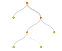
Bagging combines and averages multiple models. Averaging across multiple trees reduces the variability of any one tree and reduces overfitting, which improves predictive performance. Bagging follows three simple steps:

Fig 3. The bagging process.
This process can actually be applied to any regression or classification model; however, it provides the greatest improvement for models that have high variance. For example, more stable parametric models such as linear regression and multi-adaptive regression splines tend to experience less improvement in predictive performance.
One benefit of bagging is that, on average, a bootstrap sample will contain 63% () of the training data. This leaves about 33% () of the data out of the bootstrapped sample. We call this the out-of-bag (OOB) sample. We can use the OOB observations to estimate the model’s accuracy, creating a natural cross-validation process.
ipredFitting a bagged tree model is quite simple. Instead of using rpart we use ipred::bagging. We use coob = TRUE to use the OOB sample to estimate the test error. We see that our initial estimate error is close to $3K less than the test error we achieved with our single optimal tree (36543 vs. 39145)
# make bootstrapping reproducible
set.seed(123)

# train bagged model
bagged_m1 <- bagging(
  formula = Sale_Price ~ .,
  data    = ames_train,
  coob    = TRUE
)

bagged_m1
##
## Bagging regression trees with 25 bootstrap replications
##
## Call: bagging.data.frame(formula = Sale_Price ~ ., data = ames_train,
##     coob = TRUE)
##
## Out-of-bag estimate of root mean squared error:  36543.37
One thing to note is that typically, the more trees the better. As we add more trees we are averaging over more high variance single trees. What results is that early on, we see a dramatic reduction in variance (and hence our error) and eventually the reduction in error will flatline signaling an appropriate number of trees to create a stable model. Rarely will you need more than 50 trees to stabilize the error.
By default bagging performs 25 bootstrap samples and trees but we may require more. We can assess the error versus number of trees as below. We see that the error is stabilizing at about 25 trees so we will likely not gain much improvement by simply bagging more trees.
# assess 10-50 bagged trees
ntree <- 10:50

# create empty vector to store OOB RMSE values
rmse <- vector(mode = "numeric", length = length(ntree))

for (i in seq_along(ntree)) {
  # reproducibility
  set.seed(123)

  # perform bagged model
  model <- bagging(
  formula = Sale_Price ~ .,
  data    = ames_train,
  coob    = TRUE,
  nbagg   = ntree[i]
)
  # get OOB error
  rmse[i] <- model$err
}

plot(ntree, rmse, type = 'l', lwd = 2)
abline(v = 25, col = "red", lty = "dashed")

caretBagging with ipred is quite simple; however, there are some additional benefits of bagging with caret.
Here, we perform a 10-fold cross-validated model. We see that the cross-validated RMSE is $36,477. We also assess the top 20 variables from our model. Variable importance for regression trees is measured by assessing the total amount SSE is decreased by splits over a given predictor, averaged over all m trees. The predictors with the largest average impact to SSE are considered most important. The importance value is simply the relative mean decrease in SSE compared to the most important variable (provides a 0-100 scale).
# Specify 10-fold cross validation
ctrl <- trainControl(method = "cv",  number = 10)

# CV bagged model
bagged_cv <- train(
  Sale_Price ~ .,
  data = ames_train,
  method = "treebag",
  trControl = ctrl,
  importance = TRUE
  )

# assess results
bagged_cv
## Bagged CART
##
## 2051 samples
##   80 predictor
##
## No pre-processing
## Resampling: Cross-Validated (10 fold)
## Summary of sample sizes: 1846, 1845, 1847, 1845, 1846, 1847, ...
## Resampling results:
##
##   RMSE      Rsquared   MAE
##   36477.25  0.8001783  24059.85

# plot most important variables
plot(varImp(bagged_cv), 20)
![]()
If we compare this to the test set out of sample we see that our cross-validated error estimate was very close. We have successfully reduced our error to about $35,000; however, in later tutorials we’ll see how extensions of this bagging concept (random forests and GBMs) can significantly reduce this further.
pred <- predict(bagged_cv, ames_test)
RMSE(pred, ames_test$Sale_Price)
## [1] 35262.59
Decision trees provide a very intuitive modeling approach that have several, flexible benefits. Unfortunately, they suffer from high variance; however, when you combine them with bagging you can minimize this drawback. Moreover, bagged trees provides the fundamental basis for more complex and powerful algorithms such as random forests and gradient boosting machines. To learn more I would start with the following resources listed in order of complexity: