![]() Follow me on twitter @bradleyboehmke
Follow me on twitter @bradleyboehmke
![]() Follow me on twitter @bradleyboehmke
Follow me on twitter @bradleyboehmke
 The advent of computers brought on rapid advances in the field of statistical classification, one of which is the Support Vector Machine, or SVM. The goal of an SVM is to take groups of observations and construct boundaries to predict which group future observations belong to based on their measurements. The different groups that must be separated will be called “classes”. SVMs can handle any number of classes, as well as observations of any dimension. SVMs can take almost any shape (including linear, radial, and polynomial, among others), and are generally flexible enough to be used in almost any classification endeavor that the user chooses to undertake.
In this tutorial, we will leverage the tidyverse package to perform data manipulation, the kernlab and e1071 packages to perform calculations and produce visualizations related to SVMs, and the ISLR package to load a real world data set and demonstrate the functionality of Support Vector Machines. RColorBrewer is needed to create a custom visualization of SVMs fitted using kernlab with more than 2 classes of data. In order to allow for reproducible results, we set the random number generator explicitly.
# set pseudorandom number generator
set.seed(10)

# Attach Packages
library(tidyverse)    # data manipulation and visualization
library(kernlab)      # SVM methodology
library(e1071)        # SVM methodology
library(ISLR)         # contains example data set "Khan"
library(RColorBrewer) # customized coloring of plots
The data sets used in the tutorial (with the exception of Khan) will be generated using built-in R commands. The Support Vector Machine methodology is sound for any number of dimensions, but becomes difficult to visualize for more than 2. As previously mentioned, SVMs are robust for any number of classes, but we will stick to no more than 3 for the duration of this tutorial.
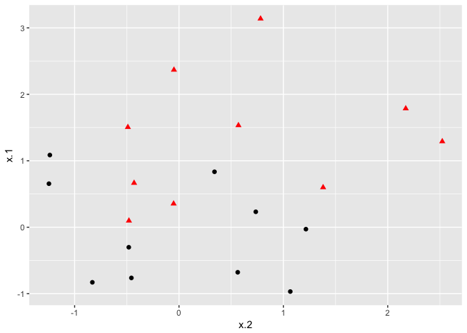
If the classes are separable by a linear boundary, we can use a Maximal Margin Classifier to find the classification boundary. To visualize an example of separated data, we generate 40 random observations and assign them to two classes. Upon visual inspection, we can see that infinitely many lines exist that split the two classes.
# Construct sample data set - completely separated
x <- matrix(rnorm(20*2), ncol = 2)
y <- c(rep(-1,10), rep(1,10))
x[y==1,] <- x[y==1,] + 3/2
dat <- data.frame(x=x, y=as.factor(y))

# Plot data
ggplot(data = dat, aes(x = x.2, y = x.1, color = y, shape = y)) +
  geom_point(size = 2) +
  scale_color_manual(values=c("#000000", "#FF0000")) +
  theme(legend.position = "none")
The goal of the maximal margin classifier is to identify the linear boundary that maximizes the total distance between the line and the closest point in each class. We can use the svm() function in the e1071 package to find this boundary.
# Fit Support Vector Machine model to data set
svmfit <- svm(y~., data = dat, kernel = "linear", scale = FALSE)
# Plot Results
plot(svmfit, dat)
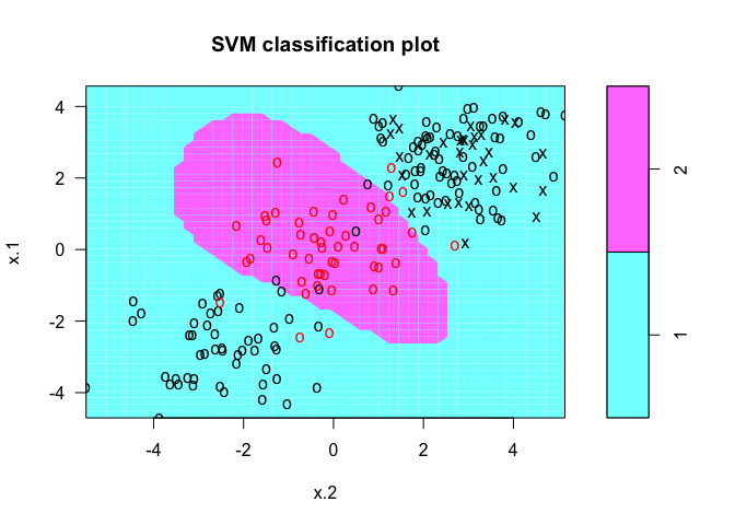
In the plot, points that are represented by an “X” are the support vectors, or the points that directly affect the classification line. The points marked with an “o” are the other points, which don’t affect the calculation of the line. This principle will lay the foundation for support vector machines. The same plot can be generated using the kernlab package, with the following results:
# fit model and produce plot
kernfit <- ksvm(x, y, type = "C-svc", kernel = 'vanilladot')
plot(kernfit, data = x)
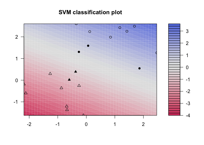
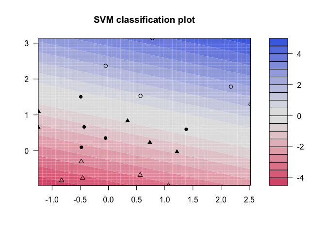
kernlab shows a little more detail than e1071, showing a color gradient that indicates how confidently a new point would be classified based on its features. Just as in the first plot, the support vectors are marked, in this case as filled-in points, while the classes are denoted by different shapes.
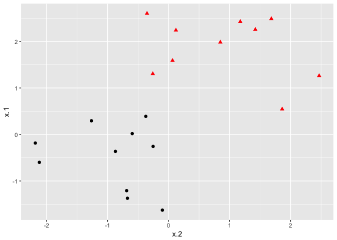
As convenient as the maximal marginal classifier is to understand, most real data sets will not be fully separable by a linear boundary. To handle such data, we must use modified methodology. We simulate a new data set where the classes are more mixed.
# Construct sample data set - not completely separated
x <- matrix(rnorm(20*2), ncol = 2)
y <- c(rep(-1,10), rep(1,10))
x[y==1,] <- x[y==1,] + 1
dat <- data.frame(x=x, y=as.factor(y))

# Plot data set
ggplot(data = dat, aes(x = x.2, y = x.1, color = y, shape = y)) +
  geom_point(size = 2) +
  scale_color_manual(values=c("#000000", "#FF0000")) +
  theme(legend.position = "none")
Whether the data is separable or not, the svm() command syntax is the same. In the case of data that is not linearly separable, however, the cost = argument takes on real importance. This quantifies the penalty associated with having an observation on the wrong side of the classification boundary. We can plot the fit in the same way as the completely separable case. We first use e1071:
# Fit Support Vector Machine model to data set
svmfit <- svm(y~., data = dat, kernel = "linear", cost = 10)
# Plot Results
plot(svmfit, dat)
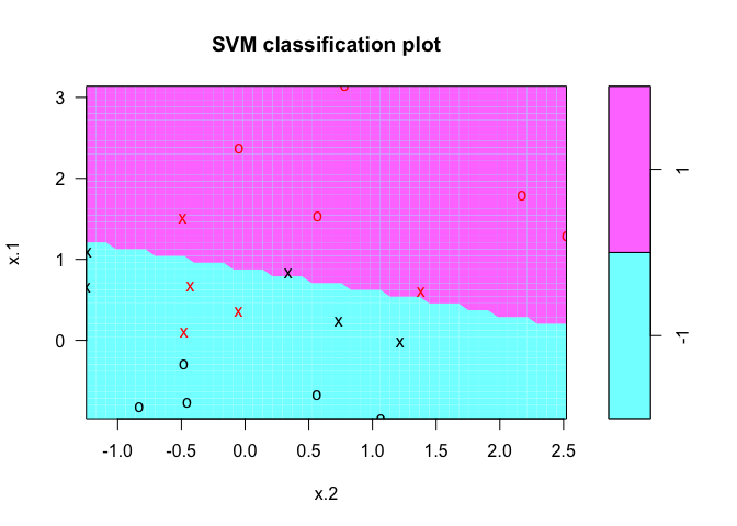
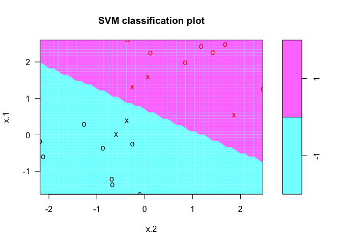
By upping the cost of misclassification from 10 to 100, you can see the difference in the classification line. We repeat the process of plotting the SVM using the kernlab package:
# Fit Support Vector Machine model to data set
kernfit <- ksvm(x,y, type = "C-svc", kernel = 'vanilladot', C = 100)
# Plot results
plot(kernfit, data = x)
But how do we decide how costly these misclassifications actually are? Instead of specifying a cost up front, we can use the tune() function from e1071 to test various costs and identify which value produces the best fitting model.
# find optimal cost of misclassification
tune.out <- tune(svm, y~., data = dat, kernel = "linear",
                 ranges = list(cost = c(0.001, 0.01, 0.1, 1, 5, 10, 100)))
# extract the best model
(bestmod <- tune.out$best.model)
##
## Call:
## best.tune(method = svm, train.x = y ~ ., data = dat, ranges = list(cost = c(0.001,
##     0.01, 0.1, 1, 5, 10, 100)), kernel = "linear")
##
##
## Parameters:
##    SVM-Type:  C-classification
##  SVM-Kernel:  linear
##        cost:  0.1
##       gamma:  0.5
##
## Number of Support Vectors:  16
For our data set, the optimal cost (from amongst the choices we provided) is calculated to be 0.1, which doesn’t penalize the model much for misclassified observations. Once this model has been identified, we can construct a table of predicted classes against true classes using the predict() command as follows:
# Create a table of misclassified observations
ypred <- predict(bestmod, dat)
(misclass <- table(predict = ypred, truth = dat$y))
##        truth
## predict -1 1
##      -1  9 3
##      1   1 7
Using this support vector classifier, 80% of the observations were correctly classified, which matches what we see in the plot. If we wanted to test our classifier more rigorously, we could split our data into training and testing sets and then see how our SVC performed with the observations not used to construct the model. We will use this training-testing method later in this tutorial to validate our SVMs.
Support Vector Classifiers are a subset of the group of classification structures known as Support Vector Machines. Support Vector Machines can construct classification boundaries that are nonlinear in shape. The options for classification structures using the svm() command from the e1071 package are linear, polynomial, radial, and sigmoid. To demonstrate a nonlinear classification boundary, we will construct a new data set.
# construct larger random data set
x <- matrix(rnorm(200*2), ncol = 2)
x[1:100,] <- x[1:100,] + 2.5
x[101:150,] <- x[101:150,] - 2.5
y <- c(rep(1,150), rep(2,50))
dat <- data.frame(x=x,y=as.factor(y))

# Plot data
ggplot(data = dat, aes(x = x.2, y = x.1, color = y, shape = y)) +
  geom_point(size = 2) +
  scale_color_manual(values=c("#000000", "#FF0000")) +
  theme(legend.position = "none")
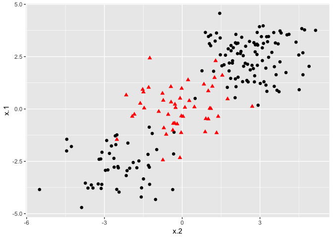
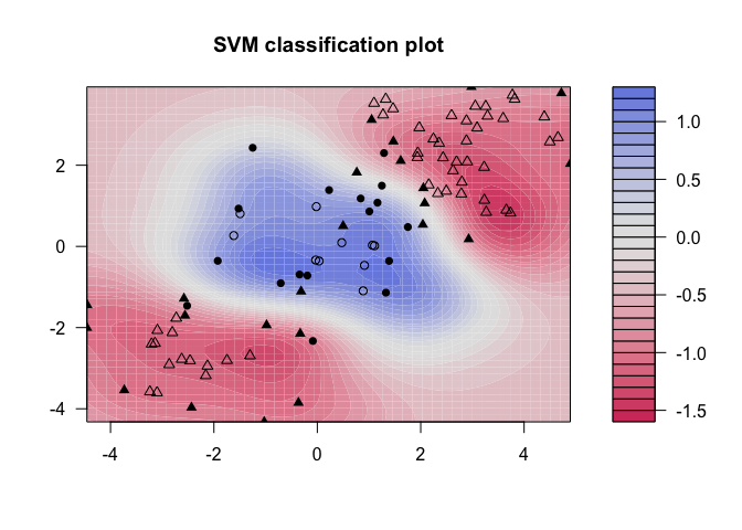
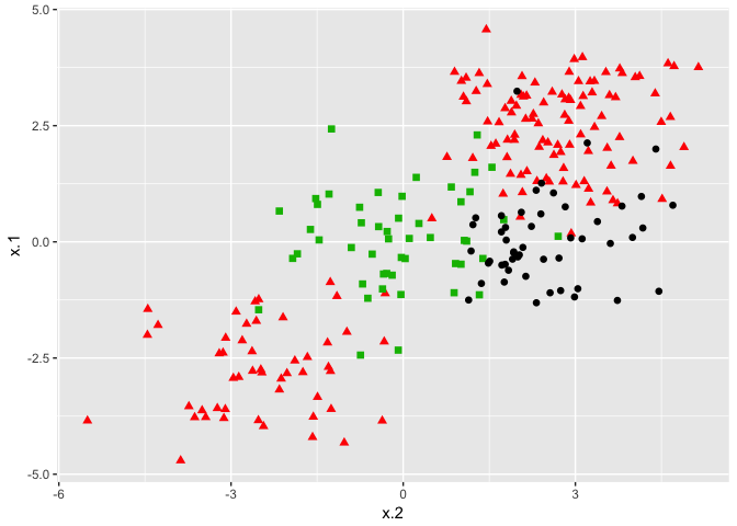
Notice that the data is not linearly separable, and furthermore, isn’t all clustered together in a single group. There are two sections of class 1 observations with a cluster of class 2 observations in between. To demonstrate the power of SVMs, we’ll take 100 random observations from the set and use them to construct our boundary. We set kernel = "radial" based on the shape of our data and plot the results.
# set pseudorandom number generator
set.seed(123)
# sample training data and fit model
train <- base::sample(200,100, replace = FALSE)
svmfit <- svm(y~., data = dat[train,], kernel = "radial", gamma = 1, cost = 1)
# plot classifier
plot(svmfit, dat)
The same procedure can be run using the kernlab package, which has far more kernel options than the corresponding function in e1071. In addition to the four choices in e1071, this package allows use of a hyperbolic tangent, Laplacian, Bessel, Spline, String, or ANOVA RBF kernel. To fit this data, we set the cost to be the same as it was before, 1.
# Fit radial-based SVM in kernlab
kernfit <- ksvm(x[train,],y[train], type = "C-svc", kernel = 'rbfdot', C = 1, scaled = c())
# Plot training data
plot(kernfit, data = x[train,])
We see that, at least visually, the SVM does a reasonable job of separating the two classes. To fit the model, we used cost = 1, but as mentioned previously, it isn’t usually obvious which cost will produce the optimal classification boundary. We can use the tune() command to try several different values of cost as well as several different values of , a scaling parameter used to fit nonlinear boundaries.
# tune model to find optimal cost, gamma values
tune.out <- tune(svm, y~., data = dat[train,], kernel = "radial",
                 ranges = list(cost = c(0.1,1,10,100,1000),
                 gamma = c(0.5,1,2,3,4)))
# show best model
tune.out$best.model
##
## Call:
## best.tune(method = svm, train.x = y ~ ., data = dat[train, ],
##     ranges = list(cost = c(0.1, 1, 10, 100, 1000), gamma = c(0.5,
##         1, 2, 3, 4)), kernel = "radial")
##
##
## Parameters:
##    SVM-Type:  C-classification
##  SVM-Kernel:  radial
##        cost:  1
##       gamma:  0.5
##
## Number of Support Vectors:  34
The model that reduces the error the most in the training data uses a cost of 1 and value of 0.5. We can now see how well the SVM performs by predicting the class of the 100 testing observations:
# validate model performance
(valid <- table(true = dat[-train,"y"], pred = predict(tune.out$best.model,
                                             newx = dat[-train,])))
##     pred
## true  1  2
##    1 58 19
##    2 16  7
Our best-fitting model produces 65% accuracy in identifying classes. For such a complicated shape of observations, this performed reasonably well. We can challenge this method further by adding additional classes of observations.
The procedure does not change for data sets that involve more than two classes of observations. We construct our data set the same way as we have previously, only now specifying three classes instead of two:
# construct data set
x <- rbind(x, matrix(rnorm(50*2), ncol = 2))
y <- c(y, rep(0,50))
x[y==0,2] <- x[y==0,2] + 2.5
dat <- data.frame(x=x, y=as.factor(y))
# plot data set
ggplot(data = dat, aes(x = x.2, y = x.1, color = y, shape = y)) +
  geom_point(size = 2) +
  scale_color_manual(values=c("#000000","#FF0000","#00BA00")) +
  theme(legend.position = "none")
The commands don’t change for the e1071 package. We specify a cost and tuning parameter and fit a support vector machine. The results and interpretation are similar to two-class classification.
# fit model
svmfit <- svm(y~., data = dat, kernel = "radial", cost = 10, gamma = 1)
# plot results
plot(svmfit, dat)
We can check to see how well our model fit the data by using the predict() command, as follows:
#construct table
ypred <- predict(svmfit, dat)
(misclass <- table(predict = ypred, truth = dat$y))
##        truth
## predict   0   1   2
##       0  38   2   4
##       1   8 143   4
##       2   4   5  42
As shown in the resulting table, 89% of our training observations were correctly classified. However, since we didn’t break our data into training and testing sets, we didn’t truly validate our results.
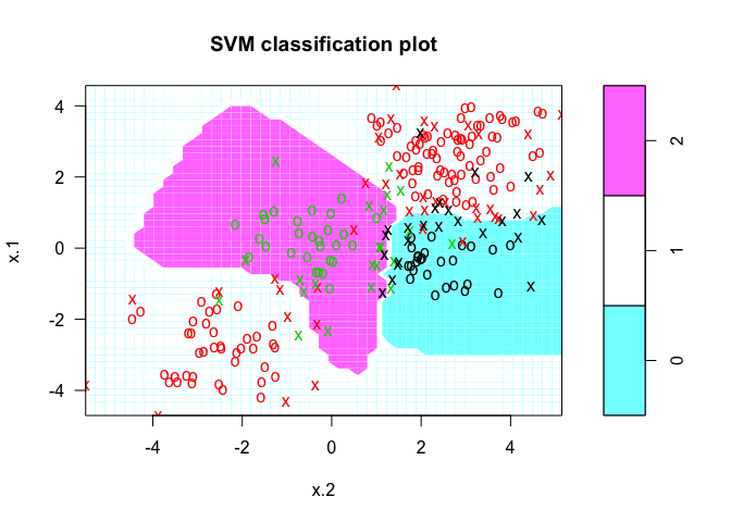
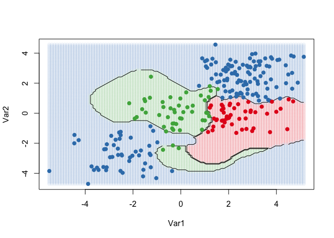
The kernlab package, on the other hand, can fit more than 2 classes, but cannot plot the results. To visualize the results of the ksvm function, we take the steps listed below to create a grid of points, predict the value of each point, and plot the results:
# fit and plot
kernfit <- ksvm(as.matrix(dat[,2:1]),dat$y, type = "C-svc", kernel = 'rbfdot',
                C = 100, scaled = c())

# Create a fine grid of the feature space
x.1 <- seq(from = min(dat$x.1), to = max(dat$x.1), length = 100)
x.2 <- seq(from = min(dat$x.2), to = max(dat$x.2), length = 100)
x.grid <- expand.grid(x.2, x.1)

# Get class predictions over grid
pred <- predict(kernfit, newdata = x.grid)

# Plot the results
cols <- brewer.pal(3, "Set1")
plot(x.grid, pch = 19, col = adjustcolor(cols[pred], alpha.f = 0.05))

classes <- matrix(pred, nrow = 100, ncol = 100)
contour(x = x.2, y = x.1, z = classes, levels = 1:3, labels = "", add = TRUE)

points(dat[, 2:1], pch = 19, col = cols[predict(kernfit)])
The Khan data set contains data on 83 tissue samples with 2308 gene expression measurements on each sample. These were split into 63 training observations and 20 testing observations, and there are four distinct classes in the set. It would be impossible to visualize such data, so we choose the simplest classifier (linear) to construct our model. We will use the svm command from e1071 to conduct our analysis.
# fit model
dat <- data.frame(x = Khan$xtrain, y=as.factor(Khan$ytrain))
(out <- svm(y~., data = dat, kernel = "linear", cost=10))
##
## Call:
## svm(formula = y ~ ., data = dat, kernel = "linear", cost = 10)
##
##
## Parameters:
##    SVM-Type:  C-classification
##  SVM-Kernel:  linear
##        cost:  10
##       gamma:  0.0004332756
##
## Number of Support Vectors:  58
First of all, we can check how well our model did at classifying the training observations. This is usually high, but again, doesn’t validate the model. If the model doesn’t do a very good job of classifying the training set, it could be a red flag. In our case, all 63 training observations were correctly classified.
# check model performance on training set
table(out$fitted, dat$y)
##
##      1  2  3  4
##   1  8  0  0  0
##   2  0 23  0  0
##   3  0  0 12  0
##   4  0  0  0 20
To perform validation, we can check how the model performs on the testing set:
# validate model performance
dat.te <- data.frame(x=Khan$xtest, y=as.factor(Khan$ytest))
pred.te <- predict(out, newdata=dat.te)
table(pred.te, dat.te$y)
##
## pred.te 1 2 3 4
##       1 3 0 0 0
##       2 0 6 2 0
##       3 0 0 4 0
##       4 0 0 0 5
The model correctly identifies 18 of the 20 testing observations. SVMs and the boundaries they impose are more difficult to interpret at higher dimensions, but these results seem to suggest that our model is a good classifier for the gene data.