![]() Follow me on twitter @bradleyboehmke
Follow me on twitter @bradleyboehmke
![]() Follow me on twitter @bradleyboehmke
Follow me on twitter @bradleyboehmke
One of the most common tests in statistics, the t-test, is used to determine whether the means of two groups are equal to each other. The assumption for the test is that both groups are sampled from normal distributions with equal variances. The null hypothesis is that the two means are equal, and the alternative is that they are not. It is known that under the null hypothesis, we can calculate a t-statistic that will follow a t-distribution with degrees of freedom. There is also a widely used modification of the t-test, known as Welch’s t-test that adjusts the number of degrees of freedom when the variances are thought not to be equal to each other. This tutorial covers the basics of performing t-tests in R.
This tutorial serves as an introduction to performing t-tests to compare two groups. First, I provide the data and packages required to replicate the analysis and then I walk through the basic operations to perform t-tests.
t.test() & wilcox.test(): The basic functions you’ll leverage for the various t-testsThis tutorial leverages the midwest data that is provided by the ggplot2 package for the one and two-sample independent t-tests. For the paired t-test I willustrate with the built in sleep data set. I also use the dplyr, tidyr, magrittr, and gridExtra packages.
library(ggplot2)        # plotting & data
library(dplyr)          # data manipulation
library(tidyr)          # data re-shaping
library(magrittr)       # pipe operator
library(gridExtra)      # provides side-by-side plotting

head(midwest)
## # A tibble: 6 x 28
##     PID    county state  area poptotal popdensity popwhite popblack
##   <int>     <chr> <chr> <dbl>    <int>      <dbl>    <int>    <int>
## 1   561     ADAMS    IL 0.052    66090  1270.9615    63917     1702
## 2   562 ALEXANDER    IL 0.014    10626   759.0000     7054     3496
## 3   563      BOND    IL 0.022    14991   681.4091    14477      429
## 4   564     BOONE    IL 0.017    30806  1812.1176    29344      127
## 5   565     BROWN    IL 0.018     5836   324.2222     5264      547
## 6   566    BUREAU    IL 0.050    35688   713.7600    35157       50
## # ... with 20 more variables: popamerindian <int>, popasian <int>,
## #   popother <int>, percwhite <dbl>, percblack <dbl>, percamerindan <dbl>,
## #   percasian <dbl>, percother <dbl>, popadults <int>, perchsd <dbl>,
## #   percollege <dbl>, percprof <dbl>, poppovertyknown <int>,
## #   percpovertyknown <dbl>, percbelowpoverty <dbl>,
## #   percchildbelowpovert <dbl>, percadultpoverty <dbl>,
## #   percelderlypoverty <dbl>, inmetro <int>, category <chr>
The t.test() function can be used to perform both one and two sample t-tests on vectors of data.
The function contains a variety of arguments and is called as follows:
 t.test(x, y = NULL, alternative = c("two.sided", "less", "greater"), mu = 0,
        paired = FALSE, var.equal = FALSE, conf.level = 0.95)
Here x is a numeric vector of data values and y is an optional numeric vector of data values. If y is excluded, the function performs a one-sample t-test on the data contained in x, if it is included it performs a two-sample t-tests using both x and y.
The mu argument provides a number indicating the true value of the mean (or difference in means if you are performing a two sample test) under the null hypothesis. By default, the test performs a two-sided t-test; however, you can perform an alternative hypothesis by changing the alternative argument to “greater” or “less” depending on whether the alternative hypothesis is that the mean is greater than or less than mu, respectively. For example the following:
t.test(x, alternative = "less", mu = 25)
…performs a one-sample t-test on the data contained in x where the null hypothesis is that and the alternative is that .
The paired argument will indicate whether or not you want a paired t-test. The default is set to FALSE but can be set to TRUE if you desire to perform a paired t-test.
The var.equal argument indicates whether or not to assume equal variances when performing a two-sample t-test. The default assumes unequal variance and applies the Welsh approximation to the degrees of freedom; however, you can set this to TRUE to pool the variance.
Finally, the conf.level argument determines the confidence level of the reported confidence interval for in the one-sample case and in the two-sample case.
The wilcox.test() function provides the same basic functionality and arguments; however, wilcox.test() is used when we do not want to assume the data to follow a normal distribution.
The one-sample t-test compares a sample’s mean with a known value, when the variance of the population is unknown. Consider we want to assess the percent of college educated adults in the midwest and compare it to a certain value. For example, let’s assume the nation-wide average of college educated adults is 32% (Bachelor’s degree or higher) and we want to see if the midwest mean is significantly different than the national average; in particular we want to test if the midwest average is less than the national average.
head(midwest$percollege, 10)
##  [1] 19.63139 11.24331 17.03382 17.27895 14.47600 18.90462 11.91739
##  [8] 16.19712 14.10765 41.29581

summary(midwest$percollege)
##    Min. 1st Qu.  Median    Mean 3rd Qu.    Max.
##   7.336  14.110  16.800  18.270  20.550  48.080
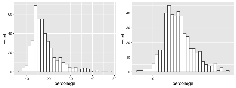
Note below the non-normality of the sample distribution which can be corrected with a log transformation. Although the Central Limit Theorem provides some robustness to the normality assumption, this is important to know so we can test our data a couple different ways to provide a comprehensive conclusion.
p1 <- ggplot(midwest, aes(percollege)) +
        geom_histogram(fill = "white", color = "grey30")

p2 <- ggplot(midwest, aes(percollege)) +
        geom_histogram(fill = "white", color = "grey30") +
        scale_x_log10()

grid.arrange(p1, p2, ncol = 2)
To test if the midwest average is less than the national average I’ll perform three tests. First I test with a normal t.test without any distribution transformations. The results below show a p-value < .001 supporting the alternative hypothesis that “the true mean is less than 32%.”
t.test(midwest$percollege, mu = 32, alternative = "less")
##
## 	One Sample t-test
##
## data:  midwest$percollege
## t = -45.827, df = 436, p-value < 2.2e-16
## alternative hypothesis: true mean is less than 32
## 95 percent confidence interval:
##     -Inf 18.7665
## sample estimates:
## mean of x
##  18.27274
Alternatively, due to the non-normality concerns we can perform this test in two additional ways to ensure our results are not being biased due to assumption violations. We can perform the test with t.test and transform our data and we can also perform the nonparametric test with the wilcox.test function. Both results support our initial conclusion that the percent of college educated adults in the midwest is statistically less than the nationwide average.
t.test(log(midwest$percollege), mu = log(32), alternative = "less")
##
## 	One Sample t-test
##
## data:  log(midwest$percollege)
## t = -41.496, df = 436, p-value < 2.2e-16
## alternative hypothesis: true mean is less than 3.465736
## 95 percent confidence interval:
##      -Inf 2.879812
## sample estimates:
## mean of x
##  2.855574

wilcox.test(midwest$percollege, mu = 32, alternative = "less")
##
## 	Wilcoxon signed rank test with continuity correction
##
## data:  midwest$percollege
## V = 924, p-value < 2.2e-16
## alternative hypothesis: true location is less than 32
Now let’s say we want to compare the differences between the average percent of college educated adults in Ohio versus Michigan. Here, we want to perform a two-sample t-test.
df <- midwest %>%
        filter(state == "OH" | state == "MI") %>%
        select(state, percollege)

# Ohio summary stats
summary(df %>% filter(state == "OH") %>% .$percollege)
##    Min. 1st Qu.  Median    Mean 3rd Qu.    Max.
##   7.913  13.090  15.460  16.890  18.990  32.200

# Michigan summary stats
summary(df %>% filter(state == "MI") %>% .$percollege)
##    Min. 1st Qu.  Median    Mean 3rd Qu.    Max.
##   11.31   14.61   17.43   19.42   21.31   48.08
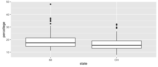
We can see Ohio appears to have slightly less college educated adults than Michigan but the graphic doesn’t tell us if it is statistically significant or not.
ggplot(df, aes(state, percollege)) +
        geom_boxplot()
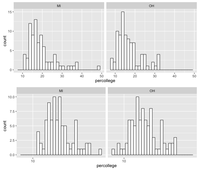
We also see similar skewness within the sample distributions.
p1 <- ggplot(df, aes(percollege)) +
        geom_histogram(fill = "white", color = "grey30") +
        facet_wrap(~ state)

p2 <- ggplot(df, aes(percollege)) +
        geom_histogram(fill = "white", color = "grey30") +
        facet_wrap(~ state) +
        scale_x_log10()

grid.arrange(p1, p2, nrow = 2)
Similar to the previous section, test if the Ohio and Michigan averages differ I’ll perform three tests. Also, note that I am searching for any differences between the means rather than if one is specifically less than or greater than the other. First I test with a normal t.test without any distribution transformations. The results below show a p-value < .01 supporting the alternative hypothesis that “true difference in means is not equal to 0”; essentially it states there is a statistical difference between the two means.
t.test(percollege ~ state, data = df)
##
## 	Welch Two Sample t-test
##
## data:  percollege by state
## t = 2.5953, df = 161.27, p-value = 0.01032
## alternative hypothesis: true difference in means is not equal to 0
## 95 percent confidence interval:
##  0.6051571 4.4568579
## sample estimates:
## mean in group MI mean in group OH
##         19.42146         16.89045
Alternatively, due to the non-normality concerns we can perform this test in two additional ways to ensure our results are not being biased due to assumption violations. We can perform the test with t.test and transform our data and we can also perform the nonparametric test with the wilcox.test function. Both results support our initial conclusion that the percent of college educated adults in Ohio is statistically different than the percent in Michigan.
t.test(log(percollege) ~ state, data = df)
##
## 	Welch Two Sample t-test
##
## data:  log(percollege) by state
## t = 2.9556, df = 168.98, p-value = 0.003567
## alternative hypothesis: true difference in means is not equal to 0
## 95 percent confidence interval:
##  0.04724892 0.23732151
## sample estimates:
## mean in group MI mean in group OH
##         2.915873         2.773587

wilcox.test(percollege ~ state, data = df)
##
## 	Wilcoxon rank sum test with continuity correction
##
## data:  percollege by state
## W = 4618, p-value = 0.002845
## alternative hypothesis: true location shift is not equal to 0
To illustrate the paired t-test I’ll use the built-in sleep data set.
sleep
##    extra group ID
## 1    0.7     1  1
## 2   -1.6     1  2
## 3   -0.2     1  3
## 4   -1.2     1  4
## 5   -0.1     1  5
## 6    3.4     1  6
## 7    3.7     1  7
## 8    0.8     1  8
## 9    0.0     1  9
## 10   2.0     1 10
## 11   1.9     2  1
## 12   0.8     2  2
## 13   1.1     2  3
## 14   0.1     2  4
## 15  -0.1     2  5
## 16   4.4     2  6
## 17   5.5     2  7
## 18   1.6     2  8
## 19   4.6     2  9
## 20   3.4     2 10

ggplot(sleep, aes(group, extra)) +
        geom_boxplot()
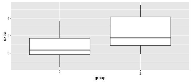
In this case we are assessing if there is a statistically significant effect of a particular drug on sleep (increase in hours of sleep compared to control) for 10 patients. See ?sleep for more details on the variables. We want to see if the mean values for the extra variable differs between group 1 and group 2. Here, we perform the t.test as in the previous sections but just add the paired = TRUE argument:
t.test(extra ~ group, data = sleep, paired = TRUE)
##
## 	Paired t-test
##
## data:  extra by group
## t = -4.0621, df = 9, p-value = 0.002833
## alternative hypothesis: true difference in means is not equal to 0
## 95 percent confidence interval:
##  -2.4598858 -0.7001142
## sample estimates:
## mean of the differences
##                   -1.58
In this example it appears that the drug does have an effect as the p-value = 0.0028 suggesting that the drug increases sleep on average by 1.58 hours.