![]() Follow me on twitter @bradleyboehmke
Follow me on twitter @bradleyboehmke
![]() Follow me on twitter @bradleyboehmke
Follow me on twitter @bradleyboehmke
 After receiving data and completing some initial data exploration, we typically move on to performing some univariate estimation and prediction tasks. A widespread tool for performing estimation and prediction is statistical inference. Statistical inference is the process of deducing properties about a population where the population is assumed to be larger than the observed data set you are currently working with. In other words, statistical inference helps you estimate parameters of a larger population when the observed data you are working with is a subset of that population. In this tutorial we examine univariate methods for statistical estimation and prediction that can provide you more confidence of your estimates when working with sample data.
This tutorial serves as an introduction to performing univariate statistical inference. First, I provide the data and packages required to replicate the analysis and then I walk through the basic operations to compute confidence intervals and perform basic hypothesis testing.
In this tutorial we’ll illustrate the key ideas using Ames, IA home sales data and employee attrition data; both provided by R packages. To illustrate the key concepts, we assume that our two data sets (ames_pop and attr_pop) represent full population data and we create samples from these populations to perform inference on.
# packages used regularly
library(dplyr)
library(ggplot2)

# full population data
ames_pop <- AmesHousing::make_ames()
attr_pop <- rsample::attrition

# reproducibility
set.seed(123)

# creating samples
ames_sample <- sample_frac(ames_pop, .5)
attr_sample <- sample_frac(attr_pop, .5)
A confidence interval estimate of a population parameter consists of an interval of numbers produced by a point estimate and an associated confidence level specifying the probability that the interval contains the parameter. Most confidence intervals take the general form
where the margin of error is a measure of the precision of the interval estimate. Smaller margin of errors indicate greater precision. Why is it important to incorporate this margin of error when working with a sample? As you can see, the mean sale price for the entire ames data set (the population) is 180,796.
mean(ames_pop$Sale_Price)
## [1] 180796.1
However, when working with subsets of this data we will get slightly different mean values. Our initial sample of the ames data, which contains 50% of the population observations, has a mean sale price of 180,873.
mean(ames_sample$Sale_Price)
## [1] 180873
If we were to grab a different sample of 50% of the population, our mean changes.
# reproducibility
set.seed(120)

# creating samples
ames_sample <- sample_frac(ames_pop, .5)
mean(ames_sample$Sale_Price)
## [1] 179101.2
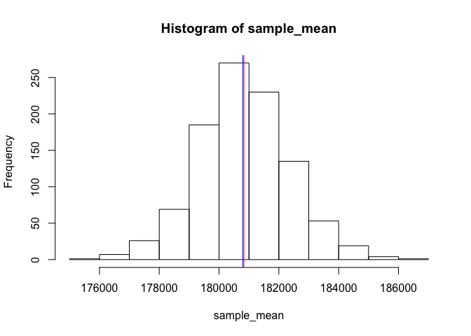
In fact, if we were able to repeat this process 1000 times, each time our sample mean would be slightly different; however, we would create a normal distribution around the estimated population mean; in this example the mean of our 1000 sample means is 180,831 with 95% confidence of being between 177,772 and 183,888. Compare this to the true population mean of 180,796.
sample_mean <- vector(mode = "double", length = 1000)

# creating 1000 sample means
for(i in seq_along(sample_mean)) {
  set.seed(i)
  sample <- sample_frac(ames_pop, .5)
  mean_stat <- mean(sample$Sale_Price)
  sample_mean[i] <- mean_stat
}

hist(sample_mean)
abline(v = mean(sample_mean), col = "red")          # average of 1000 sample means
abline(v = mean(ames_pop$Sale_Price), col = "blue") # true population mean
Unfortunately, when working with samples we typically do not have the population data to compare to so we need to estimate a confidence interval for our population mean by only using information from our sample. To compute a confidence interval we can use the t-interval, which produces reliable confidence intervals so long as our population is from a normal distribution or the sample size is large. Equation 1 represents our t-interval
where the sample mean is the point estimate and the quantity represents the margin of error. The multiplier follows a t distribution with degrees of freedom and is associated with the confidence level (i.e. 90%, 95%, 99%), which is specified by you, the analyst.
Using our original sample of the ames data, we can compute the 95% confidence interval. Note that we can use qt(.975, df = length(x) - 1) which computes .
# original ames sample data
set.seed(123)
ames_sample <- sample_frac(ames_pop, .5)

# compute equation parameters
x <- ames_sample$Sale_Price
xbar <- mean(x)                        # mean
multi <- qt(.975, df = length(x) - 1)  # multiplier
sigma <- sd(x)                         # standard deviation
denom <- sqrt(length(x))               # square root of n

# compute standard error
se <- multi * (sigma / denom)

# lower and upper confidence boundary
xbar + c(-se, se)
## [1] 176802.0 184944.1
Based on our sample data we can be 95% confident that the true population mean sales price is between $176,802 and $184,944. In our case, we know the true population mean is $180,796, which is appropriately captured by our 95% confidence interval. Consequently, when we only have sample data of a larger population we can adequately estimate the range that the true population parameter falls in with confidence intervals.
Unfortunately, R does not have a built-in function to compute mean confidence intervals. We could develop a function for this or we can just use the built-in t.test function, which provides confidence intervals along with other information we’ll cover shortly.
t.test(ames_sample$Sale_Price)
##
## 	One Sample t-test
##
## data:  ames_sample$Sale_Price
## t = 87.151, df = 1464, p-value < 0.00000000000000022
## alternative hypothesis: true mean is not equal to 0
## 95 percent confidence interval:
##  176802.0 184944.1
## sample estimates:
## mean of x
##    180873
As we saw in the last section, margin of error is represented by in Equation 1 above and determines the size of our confidence interval. The smaller the margin of error, the more precise our estimate is. Consequently, a common question is how can we reduce our margin of error? The margin of error is made up of three properties:
Consequently, we can decrease the margin of error in two ways:
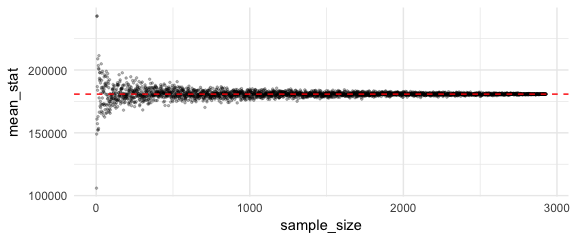
Increasing the sample size is the only way to decrease the margin of error while maintaining a constant level of confidence. In essence, increasing the sample size just means you are collecting more observations from the overall population and as you add more observations, your sample mean will be a better representation of the population mean. We can illustrate this by sampling from observations from the ames population and computing the sample mean. As the below figure demonstrates, as the sample size approaches the population size the mean values converge with the true population mean.
sample_size <- 2:nrow(ames_pop)

results <- tibble(
  sample_size = sample_size,
  mean_stat = 0
  )

for(i in seq_along(sample_size)) {
  sample <- sample_n(ames_pop, sample_size[i])
  mean_stat <- mean(sample$Sale_Price)
  results[i, 2] <- mean_stat
}

ggplot(results, aes(sample_size, mean_stat)) +
  geom_point(alpha = .25, size = .5) +
  geom_hline(yintercept = mean(ames_pop$Sale_Price), color = "red", lty = "dashed")
We can also produce confidence intervals for categorical variables. The simplest approach is to perform inference on the population proportion (). Consider the churn rate of our sample attrition data. The sample shows that 16% of sampled employees had churned (aka attrition).
attr_sample %>%
  count(Attrition) %>%
  mutate(pct = n / sum(n))
## # A tibble: 2 x 3
##   Attrition     n   pct
##   <fctr>    <int> <dbl>
## 1 No          614 0.835
## 2 Yes         121 0.165
Unfortunately, with respect to the population of our entire employee base, we have no measure of confidence in how well this sample estimate aligns with the population churn rate. In fact, it is nearly impossible that this value exactly equals . Thus, we would prefer a confidence interval for the population proportion, which can be computed with the Z-interval:
where the sample proportion p is the point estimate of and the quantity represents the margin of error. is the z value providing an area of in the upper tail of the standard normal distribution. Typical values include:
This Z-interval for may be used whenever both and . For example, a 95% confidence interval for the proportion of churners in the entire employee population is given by:
attr_sample %>%
  count(Attrition) %>%
  mutate(
    pct      = n / sum(n),
    lower.95 = pct - qnorm(.975) * sqrt((pct * (1 - pct)) / sum(n)),
    upper.95 = pct + qnorm(.975) * sqrt((pct * (1 - pct)) / sum(n))
    )
## # A tibble: 2 x 5
##   Attrition     n   pct lower.95 upper.95
##   <fctr>    <int> <dbl>    <dbl>    <dbl>
## 1 No          614 0.835    0.809    0.862
## 2 Yes         121 0.165    0.138    0.191
Now we can state that we are 95% confidence that the population attrition rate is between 13.8-19%. In fact, when we assess the population proportion in the attrition data we find that , which falls right in the middle of our estimated confidence interval.
attr_pop %>%
  count(Attrition) %>%
  mutate(pct = n / sum(n))
## # A tibble: 2 x 3
##   Attrition     n   pct
##   <fctr>    <int> <dbl>
## 1 No         1233 0.839
## 2 Yes         237 0.161
Hypothesis testing is a procedure where claims about the value of a population parameter (such as or ) may be considered using the evidence from the sample. Two competing statements, or hypotheses, are crafted about the parameter value:
Traditionally, the two possible conclusions of hypothesis testing have been (i) reject or (ii) do not reject based on the p-value (typically ). For example, a criminal trial is a form of a hypothesis test where
As the below table illustrates, there are four possible outcomes of a criminal trial with respect to the jury’s decision, and what is true in reality.
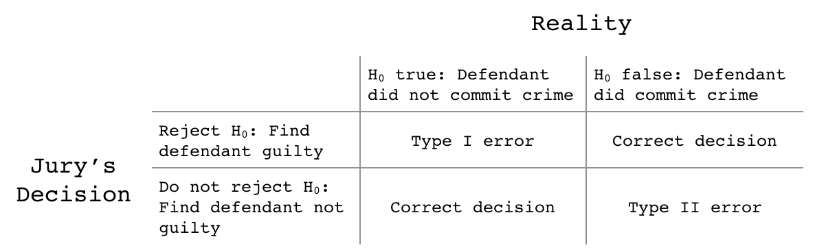
The probability of a Type I error is denoted as , while the probability of a Type II error is denoted as . For a constant sample size, a decrease in is associated with an increase in , and vice versa. In statistical inference, is usually fixed at some small value, such as 0.05, and called the level of signficance.
A common treatment of hypothesis testing for the mean is to restrict the hypotheses to the following three forms:
where represents a hypothesized value of .
When the sample size is large or the population is normally distributed, we can use t (Equation 3) as a test statistic to determine whether x deviates from the hypothesized value enough to justify rejecting the null hypothesis.
The value of t is interpreted as the number of standard errors above or below the hypothesized mean , that the sample mean resides, where the standard error equals . When t is large, it provides supporting evidence against the null hypothesis . How do we determing if we have enough supporting evidence to reject ? This is measured by the p-value.
The p-value is the probability of observing a sample statistic (such as ) at least as extreme as the statistic actually observed, if we assume is true. Thus, a p-value of 0.05 suggests there is only a 5% probability of observing if the population value is actually as suggests. Consequently, the smaller the p-value, the smaller the probability that aligns with the null hypothesis . So how small does the p-value need to be to reject ?
Historically, has been the cutoff commonly used to reject . However, it is becoming more common for data analysts to not think in terms of whether or not to reject so much as to assess the strength of evidence against the null hypothesis. The following table provides a rule-of-thumb for interpreting the strength of evidence against for various p-values.1
| p-value | Strength of Evidence Against |
|---|---|
| Extremely strong evidence | |
| Very strong evidence | |
| Solid evidence | |
| Mild evidence | |
| Slight evidence | |
| No evidence |
To perform a t-test in R we use the t.test function. For example, if we believe the average square footage of all homes sold in Ames, IA is 1,600 square feet then our hypothesis test would state:
We can test this with t.test, which shows that , which is sufficiently large. In fact, it is so large that the p-value states there is less than probability of if the population mean was 1600. This provides extremely strong evidence against . The results also tell us that the 95% confidence interval for the population mean , suggesting that the likely falls between 1468-1517 square feet.
t.test(ames_sample$Gr_Liv_Area, mu = 1600)
##
## 	One Sample t-test
##
## data:  ames_sample$Gr_Liv_Area
## t = -8.5491, df = 1464, p-value < 0.00000000000000022
## alternative hypothesis: true mean is not equal to 1600
## 95 percent confidence interval:
##  1468.272 1517.440
## sample estimates:
## mean of x
##  1492.856
We can also perform right and left-tailed tests by including the alternative argument. For example, if you owned a home in Ames, IA that had 1200 square feet on the first floor and you wanted to test if your home’s first floor square footage was larger than the average Ames home, you use alternative = "greater"2 to test, which suggests there is extremely strong evidence that your home’s first floor is larger than the average Ames, IA home’s first floor.
t.test(ames_sample$First_Flr_SF, mu = 1200, alternative = "less")
##
## 	One Sample t-test
##
## data:  ames_sample$First_Flr_SF
## t = -5.1802, df = 1464, p-value = 0.0000001263
## alternative hypothesis: true mean is less than 1200
## 95 percent confidence interval:
##      -Inf 1165.977
## sample estimates:
## mean of x
##  1150.133
Hypothesis tests may also be performed for population proportions (). The test statistic is
where is the hypothesized value of , and p is the sample proportion
The same logic applies for the z test statistic as the t test statistic. A sufficiently large z value provides evidence against the null hypothesis ; and this strength of evidence can be measured by the p-value, which can be interpreted the same as discussed in the previous section.
We can apply the prop.test function in R for hypothesis testing of proportions. For example, we can use our attr_sample data to answer the question do males and females represent and equal proportion of those employees that attrit? In this example the hypothesis is:
where the null is just testing if the proportion of females equals 50%. If this hypothesis holds then men and women are approximately equally represented. We see that in our example females represent 42% of those employees who churn. We see that our prop.test results suggest that there is extremely strong evidence that females represent less than 50% of the attrition population (its estimated that they represent 38-45% based on the 95% confidence interval). In fact, females represent 40% of the population (attr_pop) data.
# proportions table
table(attr_sample$Gender) %>% prop.table()
##
##    Female      Male
## 0.4176871 0.5823129

# hypothesis test for proportions
table(attr_sample$Gender) %>%
  prop.test()
##
## 	1-sample proportions test with continuity correction
##
## data:  ., null probability 0.5
## X-squared = 19.592, df = 1, p-value = 0.000009588
## alternative hypothesis: true p is not equal to 0.5
## 95 percent confidence interval:
##  0.3818827 0.4543636
## sample estimates:
##         p
## 0.4176871
It is important to note that prop.test will use the first proportion in the output of table to compute the z-test. Consequently, if you assumed that males represent more than 50% of those that churn you just need to reverse the table order.
table(attr_sample$Gender) %>%
  rev() %>%
  prop.test(alternative = "greater")
##
## 	1-sample proportions test with continuity correction
##
## data:  ., null probability 0.5
## X-squared = 19.592, df = 1, p-value = 0.000004794
## alternative hypothesis: true p is greater than 0.5
## 95 percent confidence interval:
##  0.5514581 1.0000000
## sample estimates:
##         p
## 0.5823129