Simplify Your Code with %>%

Removing duplication is an important principle to keep in mind with your code; however, equally important is to keep your code efficient and readable. Efficiency is often accomplished by leveraging functions and control statements in your code. However, efficiency also includes eliminating the creation and saving of unnecessary objects that often result when you are trying to make your code more readable, clear, and explicit. Consequently, writing code that is simple, readable, and efficient is often considered contradictory. For this reason, the magrittr package is a powerful tool to have in your data wrangling toolkit.

The magrittr package was created by Stefan Milton Bache and, in Stefan’s words, has two primary aims: “to decrease development time and to improve readability and maintainability of code.” Hence, it aims to increase efficiency and improve readability; and in the process it greatly simplifies your code. The following covers the basics of the magrittr toolkit.

Pipe (%>%) Operator

The principal function provided by the magrittr package is %>%, or what’s called the “pipe” operator. This operator will forward a value, or the result of an expression, into the next function call/expression. For instance a function to filter data can be written as:

filter(data, variable == numeric_value)
or
data %>% filter(variable == numeric_value)

Both functions complete the same task and the benefit of using %>% may not be immediately evident; however, when you desire to perform multiple functions its advantage becomes obvious. For instance, if we want to filter some data, group it by categories, summarize it, and then order the summarized results we could write it out three different ways. Don’t worry, you’ll learn how to operate these specific functions in the next section.

Nested Option:

arrange(
   summarize(
       group_by(
           filter(mtcars, carb > 1),
           cyl
          ),
       Avg_mpg = mean(mpg)
      ),
   desc(Avg_mpg)
 )
## Source: local data frame [3 x 2]
## 
##     cyl Avg_mpg
##   (dbl)   (dbl)
## 1     4   25.90
## 2     6   19.74
## 3     8   15.10

This first option is considered a “nested” option such that functions are nested within one another. Historically, this has been the traditional way of integrating code; however, it becomes extremely difficult to read what exactly the code is doing and it also becomes easier to make mistakes when making updates to your code. Although not in violation of the DRY principle¹, it definitely violates the basic principle of readability and clarity, which makes communication of your analysis more difficult. To make things more readable, people often move to the following approach…

Multiple Object Option:

a <- filter(mtcars, carb > 1)
b <- group_by(a, cyl)
c <- summarise(b, Avg_mpg = mean(mpg))
d <- arrange(c, desc(Avg_mpg))
print(d)
## Source: local data frame [3 x 2]
## 
##     cyl Avg_mpg
##   (dbl)   (dbl)
## 1     4   25.90
## 2     6   19.74
## 3     8   15.10

This second option helps in making the data wrangling steps more explicit and obvious but definitely violates the DRY principle. By sequencing multiple functions in this way you are likely saving multiple outputs that are not very informative to you or others; rather, the only reason you save them is to insert them into the next function to eventually get the final output you desire. This inevitably creates unnecessary copies and wrecks havoc on properly managing your objects…basically it results in a global environment charlie foxtrot! To provide the same readability (or even better), we can use %>% to string these arguments together without unnecessary object creation…

%>% Option:

library(magrittr)
library(dplyr)

mtcars %>%
        filter(carb > 1) %>%
        group_by(cyl) %>%
        summarise(Avg_mpg = mean(mpg)) %>%
        arrange(desc(Avg_mpg))
## Source: local data frame [3 x 2]
## 
##     cyl Avg_mpg
##   (dbl)   (dbl)
## 1     4   25.90
## 2     6   19.74
## 3     8   15.10

This final option which integrates %>% operators makes for more efficient and legible code. Its efficient in that it doesn’t save unncessary objects (as in option 2) and performs as effectively (as both option 1 & 2) but makes your code more readable in the process. Its legible in that you can read this as you would read normal prose (we read the %>% as “and then”): “take mtcars and then filter and then group by and then summarize and then arrange.”

And since R is a functional programming language, meaning that everything you do is basically built on functions, you can use the pipe operator to feed into just about any argument call. For example, we can pipe into a linear regression function and then get the summary of the regression parameters. Note in this case I insert “data = .” into the lm() function. When using the %>% operator the default is the argument that you are forwarding will go in as the first argument of the function that follows the %>%. However, in some functions the argument you are forwarding does not go into the default first position. In these cases, you place “.” to signal which argument you want the forwarded expression to go to.

mtcars %>%
        filter(carb > 1) %>%
        lm(mpg ~ cyl + hp, data = .) %>%
        summary()
## 
## Call:
## lm(formula = mpg ~ cyl + hp, data = .)
## 
## Residuals:
##     Min      1Q  Median      3Q     Max 
## -4.6163 -1.4162 -0.1506  1.6181  5.2021 
## 
## Coefficients:
##             Estimate Std. Error t value Pr(>|t|)    
## (Intercept) 35.67647    2.28382  15.621 2.16e-13 ***
## cyl         -2.22014    0.52619  -4.219 0.000353 ***
## hp          -0.01414    0.01323  -1.069 0.296633    
## ---
## Signif. codes:  0 '***' 0.001 '**' 0.01 '*' 0.05 '.' 0.1 ' ' 1
## 
## Residual standard error: 2.689 on 22 degrees of freedom
## Multiple R-squared:  0.7601,	Adjusted R-squared:  0.7383 
## F-statistic: 34.85 on 2 and 22 DF,  p-value: 1.516e-07

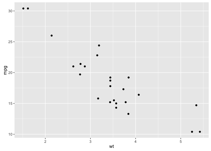
You can also use %>% to feed into plots:

library(ggplot2)

mtcars %>%
        filter(carb > 1) %>%
        qplot(x = wt, y = mpg, data = .)

You will also find that the %>% operator is now being built into packages to make programming much easier. For instance, in the tutorials where I illustrate how to reshape and transform your data with the dplyr and tidyr packages, you will see that the %>% operator is already built into these packages. It is also built into the ggvis and dygraphs packages (visualization packages), the httr package (which I covered in the data scraping tutorials), and a growing number of newer packages.

Additional Functions

In addition to the %>% operator, magrittr provides several additional functions which make operations such as addition, multiplication, logical operators, re-naming, etc. more pleasant when composing chains using the %>% operator. Some examples follow but you can see the current list of the available aliased functions by typing ?magrittr::add in your console.

# subset with extract
mtcars %>%
        extract(, 1:4) %>%
        head
##                    mpg cyl disp  hp
## Mazda RX4         21.0   6  160 110
## Mazda RX4 Wag     21.0   6  160 110
## Datsun 710        22.8   4  108  93
## Hornet 4 Drive    21.4   6  258 110
## Hornet Sportabout 18.7   8  360 175
## Valiant           18.1   6  225 105

# add, subtract, multiply, divide and other operations are available
mtcars %>% 
        extract(, "mpg") %>% 
        multiply_by(5)
##  [1] 105.0 105.0 114.0 107.0  93.5  90.5  71.5 122.0 114.0  96.0  89.0
## [12]  82.0  86.5  76.0  52.0  52.0  73.5 162.0 152.0 169.5 107.5  77.5
## [23]  76.0  66.5  96.0 136.5 130.0 152.0  79.0  98.5  75.0 107.0

# logical assessments and filters are available
mtcars %>% 
        extract(, "cyl") %>% 
        equals(4)
##  [1] FALSE FALSE  TRUE FALSE FALSE FALSE FALSE  TRUE  TRUE FALSE FALSE
## [12] FALSE FALSE FALSE FALSE FALSE FALSE  TRUE  TRUE  TRUE  TRUE FALSE
## [23] FALSE FALSE FALSE  TRUE  TRUE  TRUE FALSE FALSE FALSE  TRUE

# renaming columns and rows is available
mtcars %>%
        head %>%
        set_colnames(paste("Col", 1:11, sep = ""))
##                   Col1 Col2 Col3 Col4 Col5  Col6  Col7 Col8 Col9 Col10 Col11
## Mazda RX4         21.0    6  160  110 3.90 2.620 16.46    0    1     4     4
## Mazda RX4 Wag     21.0    6  160  110 3.90 2.875 17.02    0    1     4     4
## Datsun 710        22.8    4  108   93 3.85 2.320 18.61    1    1     4     1
## Hornet 4 Drive    21.4    6  258  110 3.08 3.215 19.44    1    0     3     1
## Hornet Sportabout 18.7    8  360  175 3.15 3.440 17.02    0    0     3     2
## Valiant           18.1    6  225  105 2.76 3.460 20.22    1    0     3     1

Additional Pipe Operators

magrittr also offers some alternative pipe operators. Some functions, such as plotting functions, will cause the string of piped arguments to terminate. The tee (%T>%) operator allows you to continue piping functions that normally cause termination.

# normal piping terminates with the plot() function resulting in
# NULL results for the summary() function
mtcars %>%
        filter(carb > 1) %>%
        extract(, 1:4) %>%
        plot() %>%
        summary()

## Length  Class   Mode 
##      0   NULL   NULL

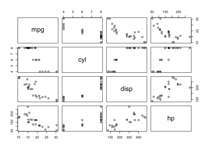
# inserting %T>% allows you to plot and perform the functions that 
# follow the plotting function
mtcars %>%
        filter(carb > 1) %>%
        extract(, 1:4) %T>%
        plot() %>%
        summary()

##       mpg             cyl            disp             hp       
##  Min.   :10.40   Min.   :4.00   Min.   : 75.7   Min.   : 52.0  
##  1st Qu.:15.20   1st Qu.:6.00   1st Qu.:146.7   1st Qu.:110.0  
##  Median :17.80   Median :8.00   Median :275.8   Median :175.0  
##  Mean   :18.62   Mean   :6.64   Mean   :257.7   Mean   :163.7  
##  3rd Qu.:21.00   3rd Qu.:8.00   3rd Qu.:351.0   3rd Qu.:205.0  
##  Max.   :30.40   Max.   :8.00   Max.   :472.0   Max.   :335.0

The compound assignment %<>% operator is used to update a value by first piping it into one or more expressions, and then assigning the result. For instance, let’s say you want to transform the mpg variable in the mtcars data frame to a square root measurement. Using %<>% will perform the functions to the right of %<>% and save the changes these functions perform to the variable or data frame called to the left of %<>%.

# note that mpg is in its typical measurement
head(mtcars)
##                    mpg cyl disp  hp drat    wt  qsec vs am gear carb
## Mazda RX4         21.0   6  160 110 3.90 2.620 16.46  0  1    4    4
## Mazda RX4 Wag     21.0   6  160 110 3.90 2.875 17.02  0  1    4    4
## Datsun 710        22.8   4  108  93 3.85 2.320 18.61  1  1    4    1
## Hornet 4 Drive    21.4   6  258 110 3.08 3.215 19.44  1  0    3    1
## Hornet Sportabout 18.7   8  360 175 3.15 3.440 17.02  0  0    3    2
## Valiant           18.1   6  225 105 2.76 3.460 20.22  1  0    3    1

# we can square root mpg and save this change using %<>%
mtcars$mpg %<>% sqrt

head(mtcars)
##                        mpg cyl disp  hp drat    wt  qsec vs am gear carb
## Mazda RX4         4.582576   6  160 110 3.90 2.620 16.46  0  1    4    4
## Mazda RX4 Wag     4.582576   6  160 110 3.90 2.875 17.02  0  1    4    4
## Datsun 710        4.774935   4  108  93 3.85 2.320 18.61  1  1    4    1
## Hornet 4 Drive    4.626013   6  258 110 3.08 3.215 19.44  1  0    3    1
## Hornet Sportabout 4.324350   8  360 175 3.15 3.440 17.02  0  0    3    2
## Valiant           4.254409   6  225 105 2.76 3.460 20.22  1  0    3    1

Some functions (e.g. lm, aggregate, cor) have a data argument, which allows the direct use of names inside the data as part of the call. The exposition (%$%) operator is useful when you want to pipe a dataframe, which may contain many columns, into a function that is only applied to some of the columns. For example, the correlation (cor) function only requires an x and y argument so if you pipe the mtcars data into the cor function using %>% you will get an error because cor doesn’t know how to handle mtcars. However, using %$% allows you to say “take this dataframe and then perform cor() on these specified columns within mtcars.”

# regular piping results in an error
mtcars %>%
        subset(vs == 0) %>%
        cor(mpg, wt)
## Error in pmatch(use, c("all.obs", "complete.obs", "pairwise.complete.obs", : object 'wt' not found

# using %$% allows you to specify variables of interest
mtcars %>%
        subset(vs == 0) %$%
        cor(mpg, wt)
## [1] -0.830671

Additional Resources

The magrittr package and its pipe operators are a great tool for making your code simple, efficient, and readable. There are limitations, or at least suggestions, on when and how you should use the operators. Garrett Grolemund and Hadley Wickham offer some advice on the proper use of pipe operators in their R for Data Science book. However, the %>% has greatly transformed our ability to write “simplified” code in R. As the pipe gains in popularity you will likely find it in more future packages and being familiar will likely result in better communication of your code.

Some additional resources regarding magrittr and the pipe operators you may find useful:

• The magrittr vignette (vignette("magrittr")) in your console) provides additional examples of using pipe operators and functions provided by magrittr.
• A blog post by Stefan Milton Bache regarding the past, present and future of magrittr
• magrittr questions on Stack Overflow
• The ensurer package, also written by Stefan Milton Bache, provides a useful way of verifying and validating data outputs in a sequence of pipe operators.