![]() Follow me on twitter @bradleyboehmke
Follow me on twitter @bradleyboehmke
![]() Follow me on twitter @bradleyboehmke
Follow me on twitter @bradleyboehmke
 Gradient boosted machines (GBMs) are an extremely popular machine learning algorithm that have proven successful across many domains and is one of the leading methods for winning Kaggle competitions. Whereas random forests build an ensemble of deep independent trees, GBMs build an ensemble of shallow and weak successive trees with each tree learning and improving on the previous. When combined, these many weak successive trees produce a powerful “committee” that are often hard to beat with other algorithms. This tutorial will cover the fundamentals of GBMs for regression problems.
This tutorial serves as an introduction to the GBMs. This tutorial will cover the following material:
gbm packagexgboost packageh2o packageThis tutorial leverages the following packages. Some of these packages play a supporting role; however, we demonstrate how to implement GBMs with several different packages and discuss the pros and cons to each.
library(rsample)      # data splitting
library(gbm)          # basic implementation
library(xgboost)      # a faster implementation of gbm
library(caret)        # an aggregator package for performing many machine learning models
library(h2o)          # a java-based platform
library(pdp)          # model visualization
library(ggplot2)      # model visualization
library(lime)         # model visualization
To illustrate various GBM concepts we will use the Ames Housing data that has been included in the AmesHousing package.
# Create training (70%) and test (30%) sets for the AmesHousing::make_ames() data.
# Use set.seed for reproducibility

set.seed(123)
ames_split <- initial_split(AmesHousing::make_ames(), prop = .7)
ames_train <- training(ames_split)
ames_test  <- testing(ames_split)
Important note: tree-based methods tend to perform well on unprocessed data (i.e. without normalizing, centering, scaling features). In this tutorial I focus on how to implement GBMs with various packages. Although I do not pre-process the data, realize that you can improve model performance by spending time processing variable attributes.
Advantages:
Disdvantages:
Several supervised machine learning models are founded on a single predictive model (i.e. linear regression, penalized models, naive Bayes, support vector machines). Alternatively, other approaches such as bagging and random forests are built on the idea of building an ensemble of models where each individual model predicts the outcome and then the ensemble simply averages the predicted values. The family of boosting methods is based on a different, constructive strategy of ensemble formation.
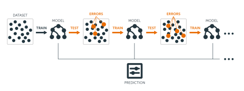
The main idea of boosting is to add new models to the ensemble sequentially. At each particular iteration, a new weak, base-learner model is trained with respect to the error of the whole ensemble learnt so far.
Let’s discuss each component of the previous sentence in closer detail because they are important.
Base-learning models: Boosting is a framework that iteratively improves any weak learning model. Many gradient boosting applications allow you to “plug in” various classes of weak learners at your disposal. In practice however, boosted algorithms almost always use decision trees as the base-learner. Consequently, this tutorial will discuss boosting in the context of regression trees.
Training weak models: A weak model is one whose error rate is only slightly better than random guessing. The idea behind boosting is that each sequential model builds a simple weak model to slightly improve the remaining errors. With regards to decision trees, shallow trees represent a weak learner. Commonly, trees with only 1-6 splits are used. Combining many weak models (versus strong ones) has a few benefits:
Sequential training with respect to errors: Boosted trees are grown sequentially; each tree is grown using information from previously grown trees. The basic algorithm for boosted regression trees can be generalized to the following where x represents our features and y represents our response:
The basic algorithm for boosted regression trees can be generalized to the following where the final model is simply a stagewise additive model of b individual regression trees:
To illustrate the behavior, assume the following x and y observations. The blue sine wave represents the true underlying function and the points represent observations that include some irriducible error (noise). The boosted prediction illustrates the adjusted predictions after each additional sequential tree is added to the algorithm. Initially, there are large errors which the boosted algorithm improves upon immediately but as the predictions get closer to the true underlying function you see each additional tree make small improvements in different areas across the feature space where errors remain. Towards the end of the gif, the predicted values nearly converge to the true underlying function.
Many algorithms, including decision trees, focus on minimizing the residuals and, therefore, emphasize the MSE loss function. The algorithm discussed in the previous section outlines the approach of sequentially fitting regression trees to minimize the errors. This specific approach is how gradient boosting minimizes the mean squared error (MSE) loss function. However, often we wish to focus on other loss functions such as mean absolute error (MAE) or to be able to apply the method to a classification problem with a loss function such as deviance. The name gradient boosting machines come from the fact that this procedure can be generalized to loss functions other than MSE.
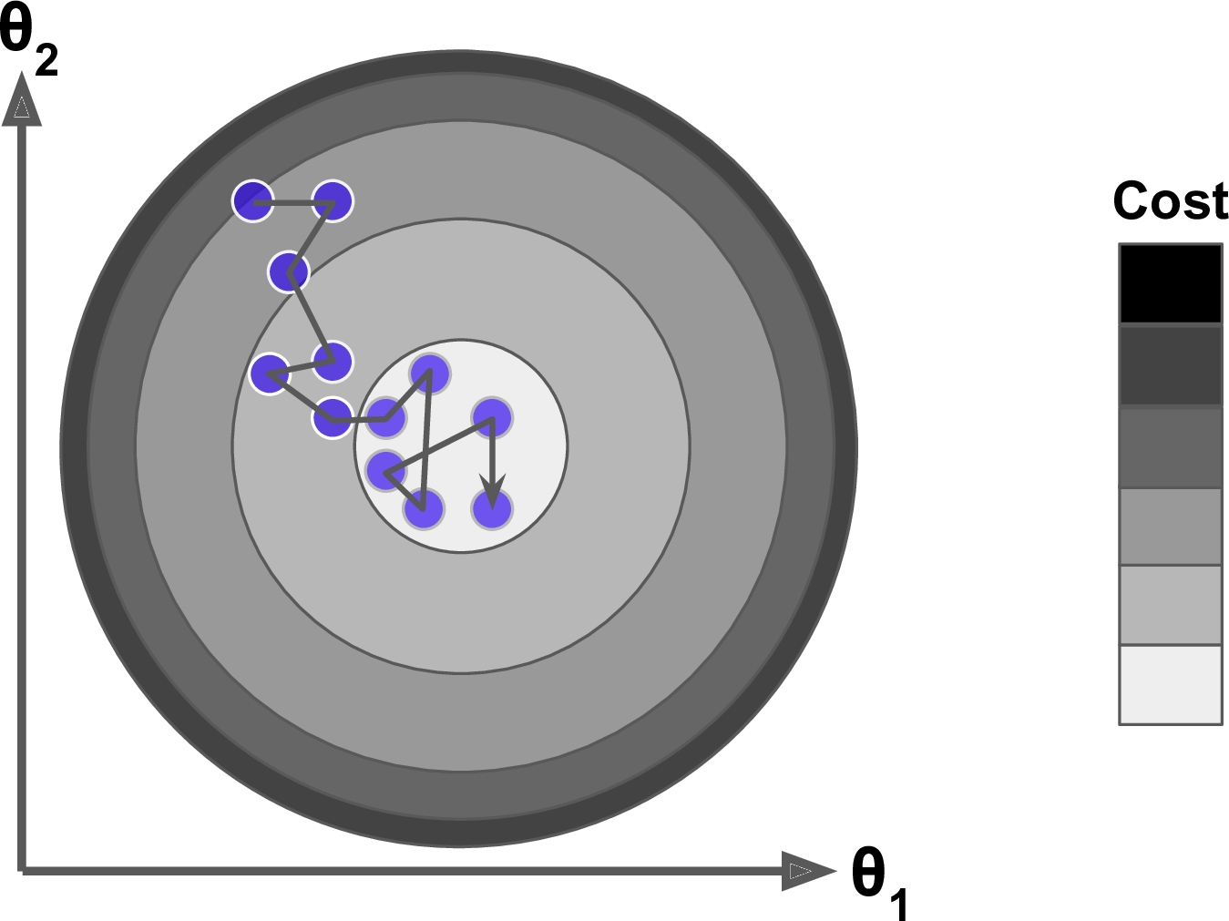
Gradient boosting is considered a gradient descent algorithm. Gradient descent is a very generic optimization algorithm capable of finding optimal solutions to a wide range of problems. The general idea of gradient descent is to tweak parameters iteratively in order to minimize a cost function. Suppose you are a downhill skier racing your friend. A good strategy to beat your friend to the bottom is to take the path with the steepest slope. This is exactly what gradient descent does - it measures the local gradient of the loss (cost) function for a given set of parameters () and takes steps in the direction of the descending gradient. Once the gradient is zero, we have reached the minimum.
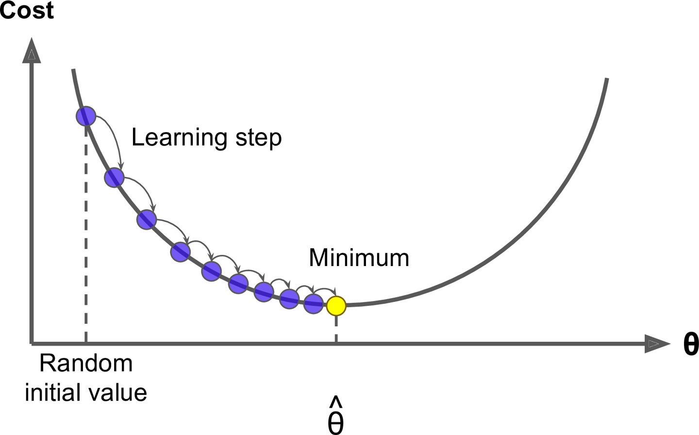
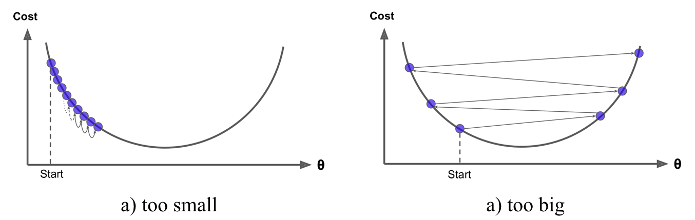
Gradient descent can be performed on any loss function that is differentiable. Consequently, this allows GBMs to optimize different loss functions as desired (see ESL, p. 360 for common loss functions). An important parameter in gradient descent is the size of the steps which is determined by the learning rate. If the learning rate is too small, then the algorithm will take many iterations to find the minimum. On the other hand, if the learning rate is too high, you might jump cross the minimum and end up further away than when you started.
Moreover, not all cost functions are convex (bowl shaped). There may be local minimas, plateaus, and other irregular terrain of the loss function that makes finding the global minimum difficult. Stochastic gradient descent can help us address this problem by sampling a fraction of the training observations (typically without replacement) and growing the next tree using that subsample. This makes the algorithm faster but the stochastic nature of random sampling also adds some random nature in descending the loss function gradient. Although this randomness does not allow the algorithm to find the absolute global minimum, it can actually help the algorithm jump out of local minima and off plateaus and get near the global minimum.
As we’ll see in the next section, there are several hyperparameter tuning options that allow us to address how we approach the gradient descent of our loss function.
Part of the beauty and challenges of GBM is that they offer several tuning parameters. The beauty in this is GBMs are highly flexible. The challenge is that they can be time consuming to tune and find the optimal combination of hyperparamters. The most common hyperparameters that you will find in most GBM implementations include:
Throughout this tutorial you’ll be exposed to additional hyperparameters that are specific to certain packages and can improve performance and/or the efficiency of training and tuning models.
There are many packages that implement GBMs and GBM variants. You can find a fairly comprehensive list here and at the CRAN Machine Learning Task View. However, the most popular implementations which we will cover in this post include:
The gbm R package is an implementation of extensions to Freund and Schapire’s AdaBoost algorithm and Friedman’s gradient boosting machine. This is the original R implementation of GBM. A presentation is available here by Mark Landry.
Features include1:
gbm has two primary training functions - gbm::gbm and gbm::gbm.fit. The primary difference is that gbm::gbm uses the formula interface to specify your model whereas gbm::gbm.fit requires the separated x and y matrices. When working with many variables it is more efficient to use the matrix rather than formula interface.
The default settings in gbm includes a learning rate (shrinkage) of 0.001. This is a very small learning rate and typically requires a large number of trees to find the minimum MSE. However, gbm uses a default number of trees of 100, which is rarely sufficient. Consequently, I crank it up to 10,000 trees. The default depth of each tree (interaction.depth) is 1, which means we are ensembling a bunch of stumps. Lastly, I also include cv.folds to perform a 5 fold cross validation. The model took about 90 seconds to run and the results show that our MSE loss function is minimized with 10,000 trees.
# for reproducibility
set.seed(123)

# train GBM model
gbm.fit <- gbm(
  formula = Sale_Price ~ .,
  distribution = "gaussian",
  data = ames_train,
  n.trees = 10000,
  interaction.depth = 1,
  shrinkage = 0.001,
  cv.folds = 5,
  n.cores = NULL, # will use all cores by default
  verbose = FALSE
  )

# print results
print(gbm.fit)
## gbm(formula = Sale_Price ~ ., distribution = "gaussian", data = ames_train,
##     n.trees = 10000, interaction.depth = 1, shrinkage = 0.001,
##     cv.folds = 5, verbose = FALSE, n.cores = NULL)
## A gradient boosted model with gaussian loss function.
## 10000 iterations were performed.
## The best cross-validation iteration was 10000.
## There were 80 predictors of which 45 had non-zero influence.
The output object is a list containing several modelling and results information. We can access this information with regular indexing; I recommend you take some time to dig around in the object to get comfortable with its components. Here, we see that the minimum CV RMSE is 29133 (this means on average our model is about $29,133 off from the actual sales price) but the plot also illustrates that the CV error is still decreasing at 10,000 trees.
# get MSE and compute RMSE
sqrt(min(gbm.fit$cv.error))
## [1] 29133.33

# plot loss function as a result of n trees added to the ensemble
gbm.perf(gbm.fit, method = "cv")
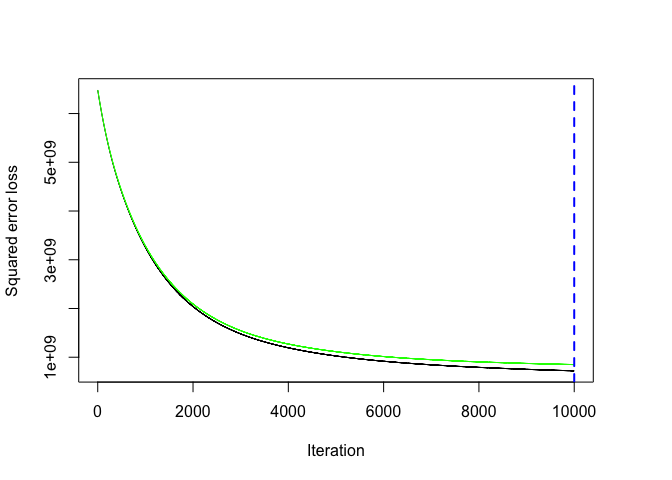
## [1] 10000
In this case, the small learning rate is resulting in very small incremental improvements which means many trees are required. In fact, for the default learning rate and tree depth settings it takes 39,906 trees for the CV error to minimize (~ 5 minutes of run time)!
However, rarely do the default settings suffice. We could tune parameters one at a time to see how the results change. For example, here, I increase the learning rate to take larger steps down the gradient descent, reduce the number of trees (since we are reducing the learning rate), and increase the depth of each tree from using a single split to 3 splits. This model takes about 90 seconds to run and achieves a significantly lower RMSE than our initial model with only 1,260 trees.
# for reproducibility
set.seed(123)

# train GBM model
gbm.fit2 <- gbm(
  formula = Sale_Price ~ .,
  distribution = "gaussian",
  data = ames_train,
  n.trees = 5000,
  interaction.depth = 3,
  shrinkage = 0.1,
  cv.folds = 5,
  n.cores = NULL, # will use all cores by default
  verbose = FALSE
  )

# find index for n trees with minimum CV error
min_MSE <- which.min(gbm.fit2$cv.error)

# get MSE and compute RMSE
sqrt(gbm.fit2$cv.error[min_MSE])
## [1] 23112.1

# plot loss function as a result of n trees added to the ensemble
gbm.perf(gbm.fit2, method = "cv")
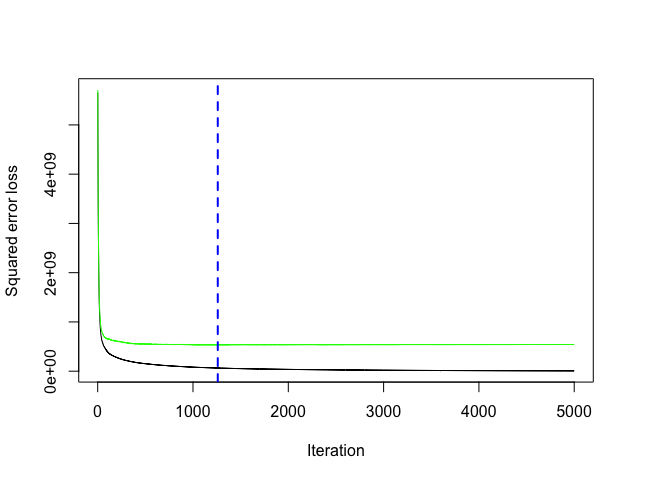
## [1] 1260
However, a better option than manually tweaking hyperparameters one at a time is to perform a grid search which iterates over every combination of hyperparameter values and allows us to assess which combination tends to perform well. To perform a manual grid search, first we want to construct our grid of hyperparameter combinations. We’re going to search across 81 models with varying learning rates and tree depth. I also vary the minimum number of observations allowed in the trees terminal nodes (n.minobsinnode) and introduce stochastic gradient descent by allowing bag.fraction < 1.
# create hyperparameter grid
hyper_grid <- expand.grid(
  shrinkage = c(.01, .1, .3),
  interaction.depth = c(1, 3, 5),
  n.minobsinnode = c(5, 10, 15),
  bag.fraction = c(.65, .8, 1),
  optimal_trees = 0,               # a place to dump results
  min_RMSE = 0                     # a place to dump results
)

# total number of combinations
nrow(hyper_grid)
## [1] 81
We loop through each hyperparameter combination and apply 5,000 trees. However, to speed up the tuning process, instead of performing 5-fold CV I train on 75% of the training observations and evaluate performance on the remaining 25%. Important note: when using train.fraction it will take the first XX% of the data so its important to randomize your rows in case their is any logic behind the ordering of the data (i.e. ordered by neighborhood).
After about 30 minutes of training time our grid search ends and we see a few important results pop out. First, our top model has better performance than our previously fitted model above, with the RMSE nearly $3,000 lower. Second, looking at the top 10 models we see that:
interaction.depth = 1); there are likely stome important interactions that the deeper trees are able to capture,bag.fraction < 1 seems to help; there may be some local minimas in our loss function gradient,n.minobsinnode = 15; the smaller nodes may allow us to capture pockets of unique feature-price point instances,# randomize data
random_index <- sample(1:nrow(ames_train), nrow(ames_train))
random_ames_train <- ames_train[random_index, ]
# grid search
for(i in 1:nrow(hyper_grid)) {
# reproducibility
set.seed(123)
# train model
gbm.tune <- gbm(
formula = Sale_Price ~ .,
distribution = "gaussian",
data = random_ames_train,
n.trees = 5000,
interaction.depth = hyper_grid$interaction.depth[i],
shrinkage = hyper_grid$shrinkage[i],
n.minobsinnode = hyper_grid$n.minobsinnode[i],
bag.fraction = hyper_grid$bag.fraction[i],
train.fraction = .75,
n.cores = NULL, # will use all cores by default
verbose = FALSE
)
# add min training error and trees to grid
hyper_grid$optimal_trees[i] <- which.min(gbm.tune$valid.error)
hyper_grid$min_RMSE[i] <- sqrt(min(gbm.tune$valid.error))
}
hyper_grid %>%
dplyr::arrange(min_RMSE) %>%
head(10)
## shrinkage interaction.depth n.minobsinnode bag.fraction optimal_trees min_RMSE
## 1 0.01 5 5 0.65 3867 16647.87
## 2 0.01 5 5 0.80 4209 16960.78
## 3 0.01 5 5 1.00 4281 17084.29
## 4 0.10 3 10 0.80 489 17093.77
## 5 0.01 3 5 0.80 4777 17121.26
## 6 0.01 3 10 0.80 4919 17139.59
## 7 0.01 3 5 0.65 4997 17139.88
## 8 0.01 5 10 0.80 4123 17162.60
## 9 0.01 5 10 0.65 4850 17247.72
## 10 0.01 3 10 1.00 4794 17353.36
These results help us to zoom into areas where we can refine our search. Let’s adjust our grid and zoom into closer regions of the values that appear to produce the best results in our previous grid search. This grid contains 81 combinations that we’ll search across.
# modify hyperparameter grid
hyper_grid <- expand.grid(
  shrinkage = c(.01, .05, .1),
  interaction.depth = c(3, 5, 7),
  n.minobsinnode = c(5, 7, 10),
  bag.fraction = c(.65, .8, 1),
  optimal_trees = 0,               # a place to dump results
  min_RMSE = 0                     # a place to dump results
)

# total number of combinations
nrow(hyper_grid)
## [1] 81
We can use the same for loop as before and perform our grid search. We get pretty similar results as before and, actually, our best model is the same as the best model above with an RMSE just above $20K.
# grid search
for(i in 1:nrow(hyper_grid)) {

  # reproducibility
  set.seed(123)

  # train model
  gbm.tune <- gbm(
    formula = Sale_Price ~ .,
    distribution = "gaussian",
    data = random_ames_train,
    n.trees = 6000,
    interaction.depth = hyper_grid$interaction.depth[i],
    shrinkage = hyper_grid$shrinkage[i],
    n.minobsinnode = hyper_grid$n.minobsinnode[i],
    bag.fraction = hyper_grid$bag.fraction[i],
    train.fraction = .75,
    n.cores = NULL, # will use all cores by default
    verbose = FALSE
  )

  # add min training error and trees to grid
  hyper_grid$optimal_trees[i] <- which.min(gbm.tune$valid.error)
  hyper_grid$min_RMSE[i] <- sqrt(min(gbm.tune$valid.error))
}

hyper_grid %>%
  dplyr::arrange(min_RMSE) %>%
  head(10)
##    n.trees shrinkage interaction.depth n.minobsinnode bag.fraction optimal_trees min_RMSE
## 1     6000      0.10                 5              5         0.65           483 20407.76
## 2     6000      0.01                 5              7         0.65          4999 20598.62
## 3     6000      0.01                 5              5         0.65          4644 20608.75
## 4     6000      0.05                 5              7         0.80          1420 20614.77
## 5     6000      0.01                 7              7         0.65          4977 20762.26
## 6     6000      0.10                 3             10         0.80          1076 20822.23
## 7     6000      0.01                 7             10         0.80          4995 20830.03
## 8     6000      0.01                 7              5         0.80          4636 20830.18
## 9     6000      0.10                 3              7         0.80           949 20839.92
## 10    6000      0.01                 5             10         0.65          4980 20840.43
Once we have found our top model we train a model with those specific parameters. And since the model converged at 483 trees I train a cross validated model (to provide a more robust error estimate) with 1000 trees. The cross-validated error of ~$22K is a better representation of the error we might expect on a new unseen data set.
# for reproducibility
set.seed(123)

# train GBM model
gbm.fit.final <- gbm(
  formula = Sale_Price ~ .,
  distribution = "gaussian",
  data = ames_train,
  n.trees = 483,
  interaction.depth = 5,
  shrinkage = 0.1,
  n.minobsinnode = 5,
  bag.fraction = .65,
  train.fraction = 1,
  n.cores = NULL, # will use all cores by default
  verbose = FALSE
  )
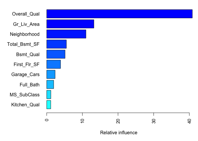
After re-running our final model we likely want to understand the variables that have the largest influence on sale price. The summary method for gbm will output a data frame and a plot that shows the most influential variables. cBars allows you to adjust the number of variables to show (in order of influence). The default method for computing variable importance is with relative influence
method = relative.influence: At each split in each tree, gbm computes the improvement in the split-criterion (MSE for regression). gbm then averages the improvement made by each variable across all the trees that the variable is used. The variables with the largest average decrease in MSE are considered most important.method = permutation.test.gbm: For each tree, the OOB sample is passed down the tree and the prediction accuracy is recorded. Then the values for each variable (one at a time) are randomly permuted and the accuracy is again computed. The decrease in accuracy as a result of this randomly “shaking up” of variable values is averaged over all the trees for each variable. The variables with the largest average decrease in accuracy are considered most important.par(mar = c(5, 8, 1, 1))
summary(
gbm.fit.final,
cBars = 10,
method = relative.influence, # also can use permutation.test.gbm
las = 2
)
##                                   var      rel.inf
## Overall_Qual             Overall_Qual 4.084734e+01
## Gr_Liv_Area               Gr_Liv_Area 1.323956e+01
## Neighborhood             Neighborhood 1.100911e+01
## Total_Bsmt_SF           Total_Bsmt_SF 5.513300e+00
## Bsmt_Qual                   Bsmt_Qual 5.149919e+00
## First_Flr_SF             First_Flr_SF 3.884696e+00
## Garage_Cars               Garage_Cars 2.354694e+00
## Full_Bath                   Full_Bath 1.953775e+00
## MS_SubClass               MS_SubClass 1.169509e+00
## Kitchen_Qual             Kitchen_Qual 1.137581e+00
...truncated...
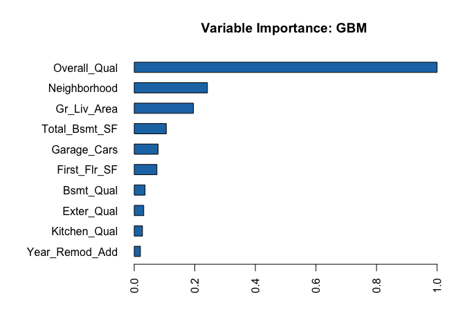
An alternative approach is to use the underdevelopment vip package, which provides ggplot2 plots. vip also provides an additional measure of variable importance based on partial dependence measures and is a common variable importance plotting framework for many machine learning models.
# devtools::install_github("koalaverse/vip")
vip::vip(gbm.fit.final)
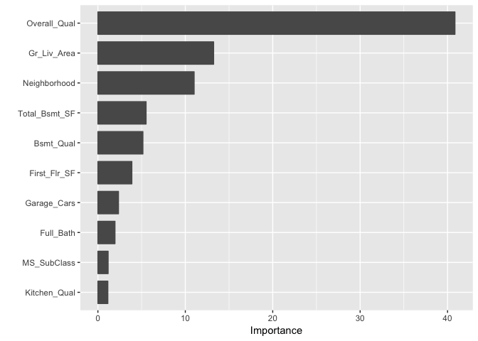
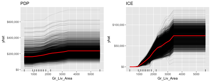
After the most relevant variables have been identified, the next step is to attempt to understand how the response variable changes based on these variables. For this we can use partial dependence plots (PDPs) and individual conditional expectation (ICE) curves.
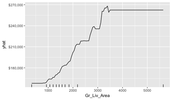
PDPs plot the change in the average predicted value as specified feature(s) vary over their marginal distribution. For example, consider the Gr_Liv_Area variable. The PDP plot below displays the average change in predicted sales price as we vary Gr_Liv_Area while holding all other variables constant. This is done by holding all variables constant for each observation in our training data set but then apply the unique values of Gr_Liv_Area for each observation. We then average the sale price across all the observations. This PDP illustrates how the predicted sales price increases as the square footage of the ground floor in a house increases.
gbm.fit.final %>%
  partial(pred.var = "Gr_Liv_Area", n.trees = gbm.fit.final$n.trees, grid.resolution = 100) %>%
  autoplot(rug = TRUE, train = ames_train) +
  scale_y_continuous(labels = scales::dollar)
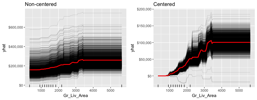
ICE curves are an extension of PDP plots but, rather than plot the average marginal effect on the response variable, we plot the change in the predicted response variable for each observation as we vary each predictor variable. Below shows the regular ICE curve plot (left) and the centered ICE curves (right). When the curves have a wide range of intercepts and are consequently “stacked” on each other, heterogeneity in the response variable values due to marginal changes in the predictor variable of interest can be difficult to discern. The centered ICE can help draw these inferences out and can highlight any strong heterogeneity in our results. The resuts show that most observations follow a common trend as Gr_Liv_Area increases; however, the centered ICE plot highlights a few observations that deviate from the common trend.
ice1 <- gbm.fit.final %>%
  partial(
    pred.var = "Gr_Liv_Area",
    n.trees = gbm.fit.final$n.trees,
    grid.resolution = 100,
    ice = TRUE
    ) %>%
  autoplot(rug = TRUE, train = ames_train, alpha = .1) +
  ggtitle("Non-centered") +
  scale_y_continuous(labels = scales::dollar)

ice2 <- gbm.fit.final %>%
  partial(
    pred.var = "Gr_Liv_Area",
    n.trees = gbm.fit.final$n.trees,
    grid.resolution = 100,
    ice = TRUE
    ) %>%
  autoplot(rug = TRUE, train = ames_train, alpha = .1, center = TRUE) +
  ggtitle("Centered") +
  scale_y_continuous(labels = scales::dollar)

gridExtra::grid.arrange(ice1, ice2, nrow = 1)
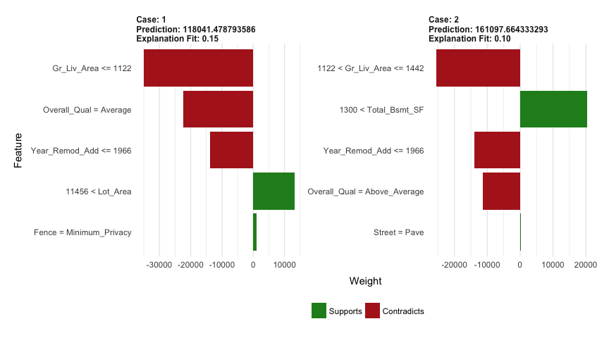
LIME is a newer procedure for understanding why a prediction resulted in a given value for a single observation. You can read more about LIME here. To use the lime package on a gbm model we need to define model type and prediction methods.
model_type.gbm <- function(x, ...) {
  return("regression")
}

predict_model.gbm <- function(x, newdata, ...) {
  pred <- predict(x, newdata, n.trees = x$n.trees)
  return(as.data.frame(pred))
}
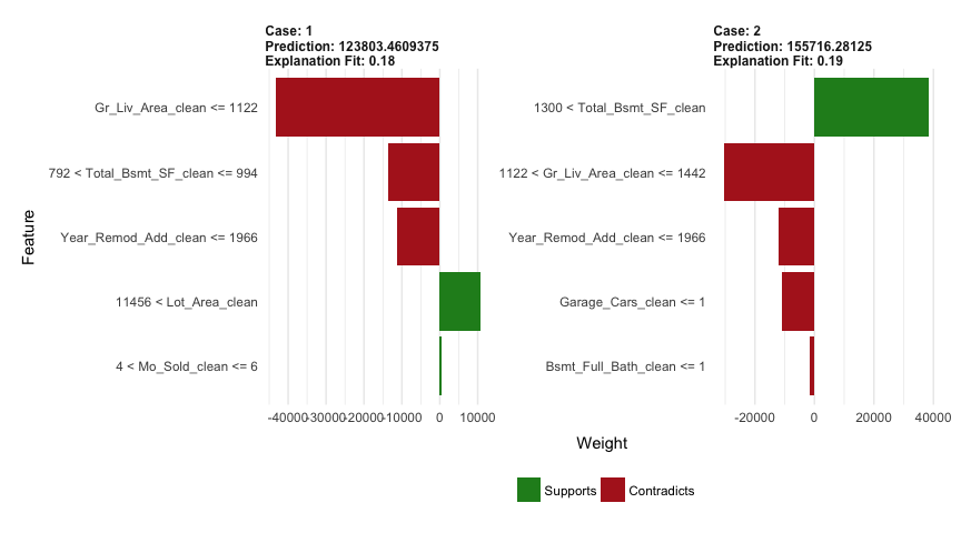
We can now apply to our two observations. The results show the predicted value (Case 1: $118K, Case 2: $161K), local model fit (both are relatively poor), and the most influential variables driving the predicted value for each observation.
# get a few observations to perform local interpretation on
local_obs <- ames_test[1:2, ]

# apply LIME
explainer <- lime(ames_train, gbm.fit.final)
explanation <- explain(local_obs, explainer, n_features = 5)
plot_features(explanation)
Once you have decided on a final model you will likely want to use the model to predict on new observations. Like most models, we simply use the predict function; however, we also need to supply the number of trees to use (see ?predict.gbm for details). We see that our RMSE for our test set is very close to the RMSE we obtained on our best gbm model.
# predict values for test data
pred <- predict(gbm.fit.final, n.trees = gbm.fit.final$n.trees, ames_test)

# results
caret::RMSE(pred, ames_test$Sale_Price)
## [1] 20681.88
The xgboost R package provides an R API to “Extreme Gradient Boosting”, which is an efficient implementation of gradient boosting framework (apprx 10x faster than gbm). The xgboost/demo repository provides a wealth of information. You can also find a fairly comprehensive parameter tuning guide here. The xgboost package has been quite popular and successful on Kaggle for data mining competitions.
Features include:
XGBoost only works with matrices that contain all numeric variables; consequently, we need to one hot encode our data. There are different ways to do this in R (i.e. Matrix::sparse.model.matrix, caret::dummyVars) but here we will use the vtreat package. vtreat is a robust package for data prep and helps to eliminate problems caused by missing values, novel categorical levels that appear in future data sets that were not in the training data, etc. However, vtreat is not very intuitive. I will not explain the functionalities but you can find more information here, here, and here.
The following applies vtreat to one-hot encode the training and testing data sets.
# variable names
features <- setdiff(names(ames_train), "Sale_Price")

# Create the treatment plan from the training data
treatplan <- vtreat::designTreatmentsZ(ames_train, features, verbose = FALSE)

# Get the "clean" variable names from the scoreFrame
new_vars <- treatplan %>%
  magrittr::use_series(scoreFrame) %>%
  dplyr::filter(code %in% c("clean", "lev")) %>%
  magrittr::use_series(varName)

# Prepare the training data
features_train <- vtreat::prepare(treatplan, ames_train, varRestriction = new_vars) %>% as.matrix()
response_train <- ames_train$Sale_Price

# Prepare the test data
features_test <- vtreat::prepare(treatplan, ames_test, varRestriction = new_vars) %>% as.matrix()
response_test <- ames_test$Sale_Price

# dimensions of one-hot encoded data
dim(features_train)
## [1] 2051  208
dim(features_test)
## [1] 879 208
xgboost provides different training functions (i.e. xgb.train which is just a wrapper for xgboost). However, to train an XGBoost we typically want to use xgb.cv, which incorporates cross-validation. The following trains a basic 5-fold cross validated XGBoost model with 1,000 trees. There are many parameters available in xgb.cv but the ones you have become more familiar with in this tutorial include the following default values:
eta): 0.3max_depth): 6min_child_weight): 1subsample –> equivalent to gbm’s bag.fraction): 100%# reproducibility
set.seed(123)
xgb.fit1 <- xgb.cv(
data = features_train,
label = response_train,
nrounds = 1000,
nfold = 5,
objective = "reg:linear", # for regression models
verbose = 0 # silent,
)
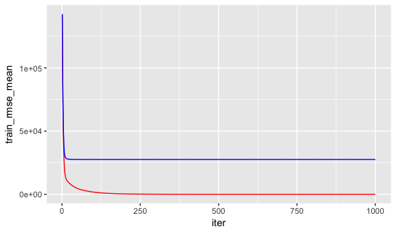
The xgb.fit1 object contains lots of good information. In particular we can assess the xgb.fit1$evaluation_log to identify the minimum RMSE and the optimal number of trees for both the training data and the cross-validated error. We can see that the training error continues to decrease to 965 trees where the RMSE nearly reaches zero; however, the cross validated error reaches a minimum RMSE of $27,572 with only 60 trees.
# get number of trees that minimize error
xgb.fit1$evaluation_log %>%
  dplyr::summarise(
    ntrees.train = which(train_rmse_mean == min(train_rmse_mean))[1],
    rmse.train   = min(train_rmse_mean),
    ntrees.test  = which(test_rmse_mean == min(test_rmse_mean))[1],
    rmse.test   = min(test_rmse_mean),
  )
##   ntrees.train rmse.train ntrees.test rmse.test
## 1          965  0.5022836          60  27572.31

# plot error vs number trees
ggplot(xgb.fit1$evaluation_log) +
  geom_line(aes(iter, train_rmse_mean), color = "red") +
  geom_line(aes(iter, test_rmse_mean), color = "blue")
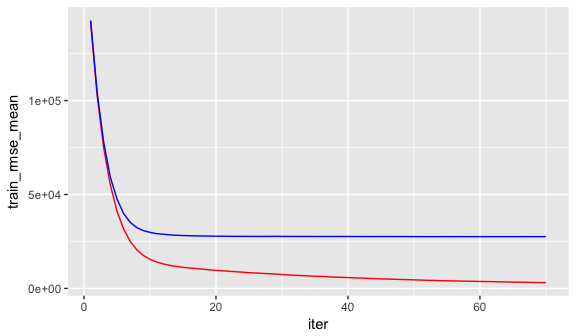
A nice feature provided by xgb.cv is early stopping. This allows us to tell the function to stop running if the cross validated error does not improve for n continuous trees. For example, the above model could be re-run with the following where we tell it stop if we see no improvement for 10 consecutive trees. This feature will help us speed up the tuning process in the next section.
# reproducibility
set.seed(123)

xgb.fit2 <- xgb.cv(
  data = features_train,
  label = response_train,
  nrounds = 1000,
  nfold = 5,
  objective = "reg:linear",  # for regression models
  verbose = 0,               # silent,
  early_stopping_rounds = 10 # stop if no improvement for 10 consecutive trees
)

# plot error vs number trees
ggplot(xgb.fit2$evaluation_log) +
  geom_line(aes(iter, train_rmse_mean), color = "red") +
  geom_line(aes(iter, test_rmse_mean), color = "blue")
To tune the XGBoost model we pass parameters as a list object to the params argument. The most common parameters include:
eta:controls the learning ratemax_depth: tree depthmin_child_weight: minimum number of observations required in each terminal nodesubsample: percent of training data to sample for each treecolsample_bytrees: percent of columns to sample from for each treeFor example, if we wanted to specify specific values for these parameters we would extend the above model with the following parameters.
# create parameter list
  params <- list(
    eta = .1,
    max_depth = 5,
    min_child_weight = 2,
    subsample = .8,
    colsample_bytree = .9
  )

# reproducibility
set.seed(123)

# train model
xgb.fit3 <- xgb.cv(
  params = params,
  data = features_train,
  label = response_train,
  nrounds = 1000,
  nfold = 5,
  objective = "reg:linear",  # for regression models
  verbose = 0,               # silent,
  early_stopping_rounds = 10 # stop if no improvement for 10 consecutive trees
)

# assess results
xgb.fit3$evaluation_log %>%
  dplyr::summarise(
    ntrees.train = which(train_rmse_mean == min(train_rmse_mean))[1],
    rmse.train   = min(train_rmse_mean),
    ntrees.test  = which(test_rmse_mean == min(test_rmse_mean))[1],
    rmse.test   = min(test_rmse_mean),
  )
##   ntrees.train rmse.train ntrees.test rmse.test
## 1          180   5891.703         170  24650.17
To perform a large search grid, we can follow the same procedure we did with gbm. We create our hyperparameter search grid along with columns to dump our results in. Here, I create a pretty large search grid consisting of 576 different hyperparameter combinations to model.
# create hyperparameter grid
hyper_grid <- expand.grid(
  eta = c(.01, .05, .1, .3),
  max_depth = c(1, 3, 5, 7),
  min_child_weight = c(1, 3, 5, 7),
  subsample = c(.65, .8, 1),
  colsample_bytree = c(.8, .9, 1),
  optimal_trees = 0,               # a place to dump results
  min_RMSE = 0                     # a place to dump results
)

nrow(hyper_grid)
## [1] 576
Now I apply the same for loop procedure to loop through and apply a XGBoost model for each hyperparameter combination and dump the results in the hyper_grid data frame. Important note: if you plan to run this code be prepared to run it before going out to eat or going to bed as it the full search grid took 6 hours to run!
# grid search
for(i in 1:nrow(hyper_grid)) {

  # create parameter list
  params <- list(
    eta = hyper_grid$eta[i],
    max_depth = hyper_grid$max_depth[i],
    min_child_weight = hyper_grid$min_child_weight[i],
    subsample = hyper_grid$subsample[i],
    colsample_bytree = hyper_grid$colsample_bytree[i]
  )

  # reproducibility
  set.seed(123)

  # train model
  xgb.tune <- xgb.cv(
    params = params,
    data = features_train,
    label = response_train,
    nrounds = 5000,
    nfold = 5,
    objective = "reg:linear",  # for regression models
    verbose = 0,               # silent,
    early_stopping_rounds = 10 # stop if no improvement for 10 consecutive trees
  )

  # add min training error and trees to grid
  hyper_grid$optimal_trees[i] <- which.min(xgb.tune$evaluation_log$test_rmse_mean)
  hyper_grid$min_RMSE[i] <- min(xgb.tune$evaluation_log$test_rmse_mean)
}

hyper_grid %>%
  dplyr::arrange(min_RMSE) %>%
  head(10)
##     eta max_depth min_child_weight subsample colsample_bytree optimal_trees min_RMSE
## 1  0.01         5                5      0.65                1          1576 23548.84
## 2  0.01         5                3      0.80                1          1626 23587.16
## 3  0.01         5                3      0.65                1          1451 23602.96
## 4  0.01         5                1      0.65                1          1480 23608.65
## 5  0.05         5                3      0.65                1           305 23743.54
## 6  0.01         5                1      0.80                1          1851 23772.90
## 7  0.05         3                3      0.65                1           552 23783.55
## 8  0.01         7                5      0.65                1          1248 23792.65
## 9  0.01         3                3      0.80                1          1923 23794.78
## 10 0.01         7                1      0.65                1          1070 23800.80
After assessing the results you would likely perform a few more grid searches to hone in on the parameters that appear to influence the model the most. In fact, here is a link to a great blog post that discusses a strategic approach to tuning with xgboost. However, for brevity, we’ll just assume the top model in the above search is the globally optimal model. Once you’ve found the optimal model, we can fit our final model with xgb.train.
# parameter list
params <- list(
  eta = 0.01,
  max_depth = 5,
  min_child_weight = 5,
  subsample = 0.65,
  colsample_bytree = 1
)

# train final model
xgb.fit.final <- xgboost(
  params = params,
  data = features_train,
  label = response_train,
  nrounds = 1576,
  objective = "reg:linear",
  verbose = 0
)
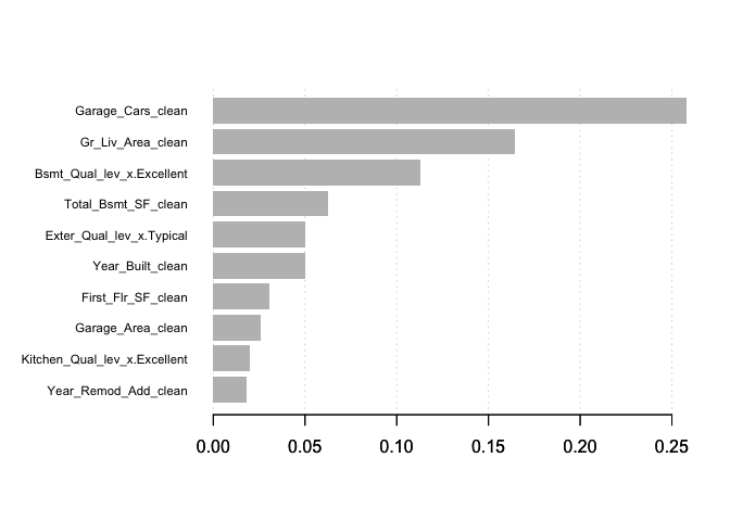
xgboost provides built-in variable importance plotting. First, you need to create the importance matrix with xgb.importance and then feed this matrix into xgb.plot.importance. There are 3 variable importance measure:
gbm’s relative.influence.# create importance matrix
importance_matrix <- xgb.importance(model = xgb.fit.final)
# variable importance plot
xgb.plot.importance(importance_matrix, top_n = 10, measure = "Gain")
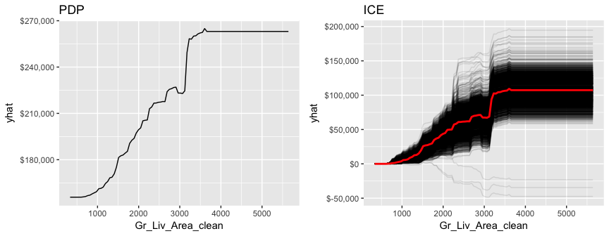
PDP and ICE plots work similarly to how we implemented them with gbm. The only difference is you need to incorporate the training data within the partial function.
pdp <- xgb.fit.final %>%
  partial(pred.var = "Gr_Liv_Area_clean", n.trees = 1576, grid.resolution = 100, train = features_train) %>%
  autoplot(rug = TRUE, train = features_train) +
  scale_y_continuous(labels = scales::dollar) +
  ggtitle("PDP")

ice <- xgb.fit.final %>%
  partial(pred.var = "Gr_Liv_Area_clean", n.trees = 1576, grid.resolution = 100, train = features_train, ice = TRUE) %>%
  autoplot(rug = TRUE, train = features_train, alpha = .1, center = TRUE) +
  scale_y_continuous(labels = scales::dollar) +
  ggtitle("ICE")

gridExtra::grid.arrange(pdp, ice, nrow = 1)
LIME provides built-in functionality for xgboost objects (see ?model_type). However, just keep in mind that the local observations being analyzed need to be one-hot encoded in the same manner as we prepared the training and test data. Also, when you feed the training data into the lime::lime function be sure that you coerce it from a matrix to a data frame.
# one-hot encode the local observations to be assessed.
local_obs_onehot <- vtreat::prepare(treatplan, local_obs, varRestriction = new_vars)

# apply LIME
explainer <- lime(data.frame(features_train), xgb.fit.final)
explanation <- explain(local_obs_onehot, explainer, n_features = 5)
plot_features(explanation)
Lastly, we use predict to predict on new observations; however, unlike gbm we do not need to provide the number of trees. Our test set RMSE is only about $600 different than that produced by our gbm model.
# predict values for test data
pred <- predict(xgb.fit.final, features_test)

# results
caret::RMSE(pred, response_test)
## [1] 21319.3
The h2o R package is a powerful and efficient java-based interface that allows for local and cluster-based deployment. It comes with a fairly comprehensive online resource that includes methodology and code documentation along with tutorials.
Features include:
Lets go ahead and start up h2o:
h2o.no_progress()
h2o.init(max_mem_size = "5g")
##  Connection successful!
##
## R is connected to the H2O cluster:
##     H2O cluster uptime:         1 days 8 hours
##     H2O cluster timezone:       America/New_York
##     H2O data parsing timezone:  UTC
##     H2O cluster version:        3.18.0.11
##     H2O cluster version age:    20 days
##     H2O cluster name:           H2O_started_from_R_bradboehmke_zvs686
##     H2O cluster total nodes:    1
##     H2O cluster total memory:   2.70 GB
##     H2O cluster total cores:    4
##     H2O cluster allowed cores:  4
##     H2O cluster healthy:        TRUE
##     H2O Connection ip:          localhost
##     H2O Connection port:        54321
##     H2O Connection proxy:       NA
##     H2O Internal Security:      FALSE
##     H2O API Extensions:         XGBoost, Algos, AutoML, Core V3, Core V4
##     R Version:                  R version 3.5.0 (2018-04-23)
h2o.gbm allows us to perform a GBM with H2O. However, prior to running our initial model we need to convert our training data to an h2o object. By default, h2o.gbm applies a GBM model with the following parameters:
ntrees): 50learn_rate): 0.1max_depth): 5min_rows): 10# create feature names
y <- "Sale_Price"
x <- setdiff(names(ames_train), y)
# turn training set into h2o object
train.h2o <- as.h2o(ames_train)
# training basic GBM model with defaults
h2o.fit1 <- h2o.gbm(
x = x,
y = y,
training_frame = train.h2o,
nfolds = 5
)
# assess model results
h2o.fit1
## Model Details:
## ==============
##
## H2ORegressionModel: gbm
## Model ID: GBM_model_R_1528813224809_1
## Model Summary:
## number_of_trees number_of_internal_trees model_size_in_bytes min_depth max_depth mean_depth min_leaves max_leaves
## 1 50 50 17360 5 5 5.00000 10 31
## mean_leaves
## 1 22.60000
##
##
## H2ORegressionMetrics: gbm
## ** Reported on training data. **
##
## MSE: 165078993
## RMSE: 12848.31
## MAE: 9243.007
## RMSLE: 0.08504509
## Mean Residual Deviance : 165078993
##
##
##
## H2ORegressionMetrics: gbm
## ** Reported on cross-validation data. **
## ** 5-fold cross-validation on training data (Metrics computed for combined holdout predictions) **
##
## MSE: 690559339
## RMSE: 26278.5
## MAE: 15706.57
## RMSLE: 0.1418509
## Mean Residual Deviance : 690559339
##
##
## Cross-Validation Metrics Summary:
## mean sd cv_1_valid cv_2_valid cv_3_valid cv_4_valid cv_5_valid
## mae 15693.389 416.34943 15772.27 14608.483 15983.741 16375.13 15727.32
## mean_residual_deviance 6.8786246E8 1.0933132E8 6.4370349E8 4.80721376E8 8.2373146E8 9.0298413E8 5.881719E8
## mse 6.8786246E8 1.0933132E8 6.4370349E8 4.80721376E8 8.2373146E8 9.0298413E8 5.881719E8
## r2 0.89403546 0.014769712 0.9059133 0.92479074 0.8778974 0.86524695 0.8963289
## residual_deviance 6.8786246E8 1.0933132E8 6.4370349E8 4.80721376E8 8.2373146E8 9.0298413E8 5.881719E8
## rmse 26059.87 2091.1375 25371.312 21925.36 28700.723 30049.693 24252.256
## rmsle 0.13967283 0.015356901 0.13289417 0.110673144 0.13735695 0.13947856 0.17796135
Similar to XGBoost, we can incorporate automated stopping so that we can crank up the number of trees but terminate training once model improvement decreases or stops. There is also an option to terminate training after so much time has passed (see max_runtime_secs). In this example, I train a default model with 5,000 trees but stop training after 10 consecutive trees have no improvement on the cross-validated error. In this case, training stops after 3828 trees and has a cross-validated RMSE of $24,684.
# training basic GBM model with defaults
h2o.fit2 <- h2o.gbm(
  x = x,
  y = y,
  training_frame = train.h2o,
  nfolds = 5,
  ntrees = 5000,
  stopping_rounds = 10,
  stopping_tolerance = 0,
  seed = 123
)

# model stopped after xx trees
h2o.fit2@parameters$ntrees
## [1] 3828

# cross validated RMSE
h2o.rmse(h2o.fit2, xval = TRUE)
## [1] 24684.09
H2O provides many parameters that can be adjusted. It is well worth your time to check out the available documentation at H2O.ai. For this tutorial, we’ll focus on the more common hyperparameters that I typically apply. This includes:
ntrees: number of trees to trainmax_depth: depth of each treemin_rows: Fewest observations allowed in a terminal nodelearn_rate: rate to descend the loss function gradientlearn_rate_annealing: allows you to have a high initial learn_rate, then gradually reduce as trees are added (speeds up training).sample_rate: row sample rate per treecol_sample_rate: column sample rate per tree (synonymous with xgboost’s colsample_bytree)Note that there are parameters that control how categorical and continuous variables are encoded, binned, and split. The defaults tend to perform quite well but I have been able to gain small improvements in certain circumstances by adjusting these. I will not cover them but they are work reviewing.
To perform grid search tuning with H2O we have two options: perform a full or random discrete grid search.
A full cartesian grid search examines every combination of hyperparameter settings that we specify in a tuning grid. This has been the type of tuning we have been performing with our manual for loops with gbm and xgboost. However, to speed up training with H2O I’ll use a validation set rather than perform k-fold cross validation. The following creates a hyperparameter grid consisting of 486 hyperparameter combinations. We apply h2o.grid to perform a grid search while also incorporating stopping parameters to reduce training time. Total grid search time was about 90 minutes.
A few characteristics pop out when we assess the results - models with trees deeper than one split with a low learning rate, no annealing, and stochastic observation sampling tend to perform best.
# create training & validation sets
split <- h2o.splitFrame(train.h2o, ratios = 0.75)
train <- split[[1]]
valid <- split[[2]]

# create hyperparameter grid
hyper_grid <- list(
  max_depth = c(1, 3, 5),
  min_rows = c(1, 5, 10),
  learn_rate = c(0.01, 0.05, 0.1),
  learn_rate_annealing = c(.99, 1),
  sample_rate = c(.5, .75, 1),
  col_sample_rate = c(.8, .9, 1)
)

# perform grid search
grid <- h2o.grid(
  algorithm = "gbm",
  grid_id = "gbm_grid1",
  x = x,
  y = y,
  training_frame = train,
  validation_frame = valid,
  hyper_params = hyper_grid,
  ntrees = 5000,
  stopping_rounds = 10,
  stopping_tolerance = 0,
  seed = 123
  )

# collect the results and sort by our model performance metric of choice
grid_perf <- h2o.getGrid(
  grid_id = "gbm_grid1",
  sort_by = "mse",
  decreasing = FALSE
  )
grid_perf
## H2O Grid Details
## ================
##
## Grid ID: gbm_grid1
## Used hyper parameters:
##   -  col_sample_rate
##   -  learn_rate
##   -  learn_rate_annealing
##   -  max_depth
##   -  min_rows
##   -  sample_rate
## Number of models: 486
## Number of failed models: 0
##
## Hyper-Parameter Search Summary: ordered by increasing mse
##   col_sample_rate learn_rate learn_rate_annealing max_depth min_rows sample_rate           model_ids                  mse
## 1             1.0       0.01                  1.0         3     10.0        0.75 gbm_grid1_model_299 3.6209830674536294E8
## 2             0.8       0.01                  1.0         3     10.0        0.75 gbm_grid1_model_297 3.6380633209494674E8
## 3             0.8       0.01                  1.0         3      1.0         0.5  gbm_grid1_model_27 3.6672773986842275E8
## 4             0.8       0.01                  1.0         5      1.0         0.5  gbm_grid1_model_45  3.683498830618852E8
## 5             0.9       0.01                  1.0         3     10.0        0.75 gbm_grid1_model_298  3.686060225554216E8
##
## ---
##     col_sample_rate learn_rate learn_rate_annealing max_depth min_rows sample_rate           model_ids                  mse
## 481             0.9       0.01                 0.99         1     10.0         1.0 gbm_grid1_model_433  2.824716768094968E9
## 482             0.9       0.01                 0.99         1      1.0         1.0 gbm_grid1_model_325  2.824716768094968E9
## 483             0.9       0.01                 0.99         1      5.0         1.0 gbm_grid1_model_379  2.824716768094968E9
## 484             1.0       0.01                 0.99         1      5.0         1.0 gbm_grid1_model_380 2.8252384874380198E9
## 485             1.0       0.01                 0.99         1      1.0         1.0 gbm_grid1_model_326 2.8252384874380198E9
## 486             1.0       0.01                 0.99         1     10.0         1.0 gbm_grid1_model_434 2.8252384874380198E9
We can check out more details of the best performing model. The top model achieves a validation RMSE of $19,029.
# Grab the model_id for the top model, chosen by validation error
best_model_id <- grid_perf@model_ids[[1]]
best_model <- h2o.getModel(best_model_id)

# Now let’s get performance metrics on the best model
h2o.performance(model = best_model, valid = TRUE)
## H2ORegressionMetrics: gbm
## ** Reported on validation data. **
##
## MSE:  362098307
## RMSE:  19028.88
## MAE:  12427.99
## RMSLE:  0.1403692
## Mean Residual Deviance :  362098307
Because of the combinatorial explosion, each additional hyperparameter that gets added to our grid search has a huge effect on the time to complete. Consequently, h2o provides an additional grid search path called “RandomDiscrete”, which will jump from one random combination to another and stop once a certain level of improvement has been made, certain amount of time has been exceeded, or a certain amount of models have been ran (or a combination of these have been met). Although using a random discrete search path will likely not find the optimal model, it typically does a good job of finding a very good model.
The following performs a random discrete grid search using the same hyperparameter grid we used above. However, in this example we add a search criteria (which is preferred when using a random search) that stops the grid search if none of the last 10 models have managed to have a 0.5% improvement in MSE compared to the best model before that. If we continue to find improvements then I cut the grid search off after 3600 seconds (60 minutes). In this example, our search went for the entire 60 minutes and evaluated 291 of the 486 potential models.
# random grid search criteria
search_criteria <- list(
  strategy = "RandomDiscrete",
  stopping_metric = "mse",
  stopping_tolerance = 0.005,
  stopping_rounds = 10,
  max_runtime_secs = 60*60
  )

# perform grid search
grid <- h2o.grid(
  algorithm = "gbm",
  grid_id = "gbm_grid2",
  x = x,
  y = y,
  training_frame = train,
  validation_frame = valid,
  hyper_params = hyper_grid,
  search_criteria = search_criteria, # add search criteria
  ntrees = 5000,
  stopping_rounds = 10,
  stopping_tolerance = 0,
  seed = 123
  )

# collect the results and sort by our model performance metric of choice
grid_perf <- h2o.getGrid(
  grid_id = "gbm_grid2",
  sort_by = "mse",
  decreasing = FALSE
  )
grid_perf
## H2O Grid Details
## ================
##
## Grid ID: gbm_grid2
## Used hyper parameters:
##   -  col_sample_rate
##   -  learn_rate
##   -  learn_rate_annealing
##   -  max_depth
##   -  min_rows
##   -  sample_rate
## Number of models: 291
## Number of failed models: 0
##
## Hyper-Parameter Search Summary: ordered by increasing mse
##   col_sample_rate learn_rate learn_rate_annealing max_depth min_rows sample_rate           model_ids                  mse
## 1             0.8       0.05                  1.0         3     10.0         1.0  gbm_grid2_model_74  5.150720254988258E8
## 2             0.9       0.01                  1.0         3      5.0         0.5 gbm_grid2_model_146 5.1889115659740096E8
## 3             0.9       0.05                  1.0         3      5.0         0.5 gbm_grid2_model_114 5.2062049083883923E8
## 4             0.8       0.05                  1.0         3      5.0        0.75  gbm_grid2_model_37 5.2124226584496534E8
## 5             0.9       0.05                  1.0         3     10.0         1.0 gbm_grid2_model_157  5.212796449846914E8
##
## ---
##     col_sample_rate learn_rate learn_rate_annealing max_depth min_rows sample_rate           model_ids                  mse
## 286             0.9       0.01                 0.99         1     10.0         1.0 gbm_grid2_model_179  3.323851889022955E9
## 287             1.0       0.01                 0.99         1     10.0         1.0 gbm_grid2_model_260 3.3243159009633546E9
## 288             0.9       0.01                 0.99         1      5.0         0.5 gbm_grid2_model_199 3.3243216930611935E9
## 289             0.8       0.01                 0.99         1     10.0         0.5  gbm_grid2_model_80 3.3244630344508557E9
## 290             0.8       0.01                 0.99         1      1.0         0.5  gbm_grid2_model_71 3.3244630344508557E9
## 291             0.8       0.01                 0.99         1      5.0         0.5 gbm_grid2_model_227 3.3244630344508557E9
In this example, the best model obtained a cross-validated RMSE of $22,695. Not quite as good as the full grid search; however, often the results come much closer.
# Grab the model_id for the top model, chosen by validation error
best_model_id <- grid_perf@model_ids[[1]]
best_model <- h2o.getModel(best_model_id)

# Now let’s get performance metrics on the best model
h2o.performance(model = best_model, valid = TRUE)
## H2ORegressionMetrics: gbm
## ** Reported on validation data. **
##
## MSE:  515072025
## RMSE:  22695.2
## MAE:  13841.13
## RMSLE:  0.1427291
## Mean Residual Deviance :  515072025
Once we’ve found our preferred model, we’ll go ahead and retrain a new model with the full training data. I’ll use the best model from the full grid search and perform a 5-fold CV to get a robust estimate of the expected error.
# train final model
h2o.final <- h2o.gbm(
  x = x,
  y = y,
  training_frame = train.h2o,
  nfolds = 5,
  ntrees = 10000,
  learn_rate = 0.01,
  learn_rate_annealing = 1,
  max_depth = 3,
  min_rows = 10,
  sample_rate = 0.75,
  col_sample_rate = 1,
  stopping_rounds = 10,
  stopping_tolerance = 0,
  seed = 123
)

# model stopped after xx trees
h2o.final@parameters$ntrees
## [1] 9385

# cross validated RMSE
h2o.rmse(h2o.final, xval = TRUE)
## [1] 23218.45
h2o provides a built function that plots variable importance. It only has one measure of variable importance, relative importance, which measures the average impact each variable has across all the trees on the loss function. The variable with the largest is most importance and the impact of all other variables are provided relative to the most important variable. The vip package also works with h2o objects to plot variable importance.
h2o.varimp_plot(h2o.final, num_of_features = 10)
We can also create similar PDP and ICE plots as before. We only need to incorporate a specialty function that converts the supplied data to an h2o object and then formats the predicted output as a data frame. We feed this into the partial function and the rest is standard.
pfun <- function(object, newdata) {
  as.data.frame(predict(object, newdata = as.h2o(newdata)))[[1L]]
}

pdp <- h2o.final %>%
  partial(
    pred.var = "Gr_Liv_Area",
    pred.fun = pfun,
    grid.resolution = 20,
    train = ames_train
    ) %>%
  autoplot(rug = TRUE, train = ames_train, alpha = .1) +
  scale_y_continuous(labels = scales::dollar) +
  ggtitle("PDP")

ice <- h2o.final %>%
  partial(
    pred.var = "Gr_Liv_Area",
    pred.fun = pfun,
    grid.resolution = 20,
    train = ames_train,
    ice = TRUE
    ) %>%
  autoplot(rug = TRUE, train = ames_train, alpha = .1, center = TRUE) +
  scale_y_continuous(labels = scales::dollar) +
  ggtitle("ICE")

gridExtra::grid.arrange(pdp, ice, nrow = 1)
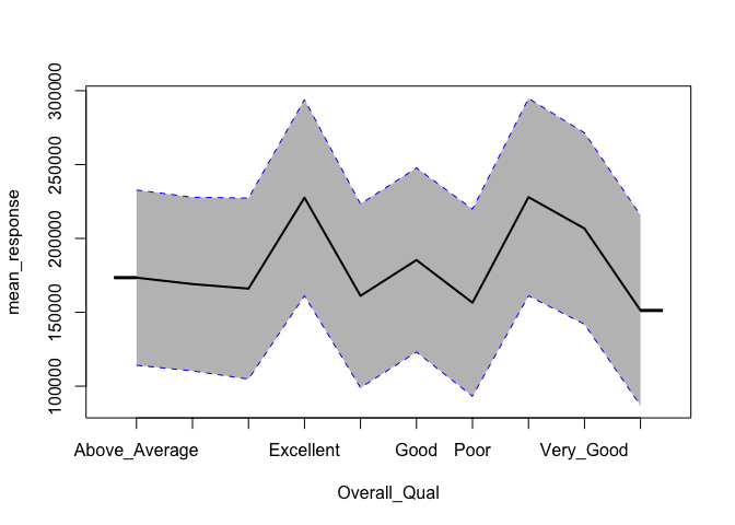
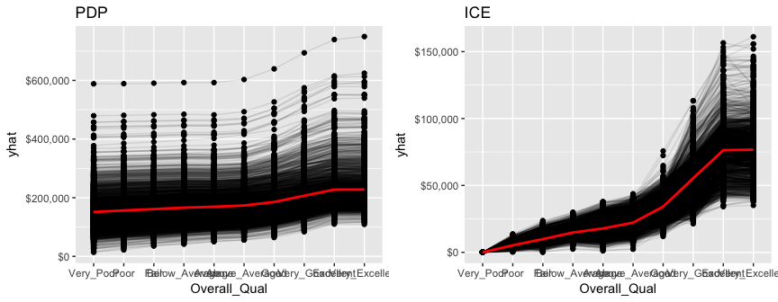
h2o does not provide built-in ICE plots but it does provide a PDP plot that plots not only the mean marginal impact (as in a normal PDP) but also one standard error to show the variability.
h2o.partialPlot(h2o.final, data = train.h2o, cols = "Overall_Qual")
## PartialDependence: Partial Dependence Plot of model GBM_model_R_1528826179077_5 on column 'Overall_Qual'
##      Overall_Qual mean_response stddev_response
## 1   Above_Average 173455.738331    59312.490353
## 2         Average 169106.725259    58783.969565
## 3   Below_Average 166036.746826    61278.387041
## 4       Excellent 227580.796151    66397.833661
## 5            Fair 161148.080639    62201.228046
## 6            Good 185388.598046    62306.233255
## 7            Poor 156493.400673    63340.558363
## 8  Very_Excellent 227965.543212    66833.666984
## 9       Very_Good 206703.390125    64790.060632
## 10      Very_Poor 151256.551340    64421.926029
Unfortunately, h2o’s function plots the categorical levels in alphabetical order whereas pdp will plot them in their specified level order making inference more intuitive.
pdp <- h2o.final %>%
  partial(
    pred.var = "Overall_Qual",
    pred.fun = pfun,
    grid.resolution = 20,
    train = as.data.frame(ames_train)
    ) %>%
  autoplot(rug = TRUE, train = ames_train, alpha = .1) +
  scale_y_continuous(labels = scales::dollar) +
  ggtitle("PDP")

ice <- h2o.final %>%
  partial(
    pred.var = "Overall_Qual",
    pred.fun = pfun,
    grid.resolution = 20,
    train = as.data.frame(ames_train),
    ice = TRUE
    ) %>%
  autoplot(rug = TRUE, train = ames_train, alpha = .1, center = TRUE) +
  scale_y_continuous(labels = scales::dollar) +
  ggtitle("ICE")

gridExtra::grid.arrange(pdp, ice, nrow = 1)
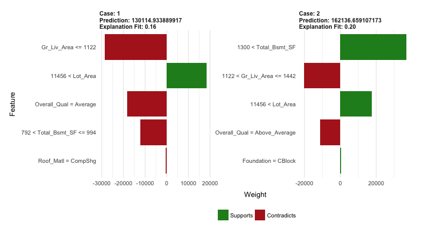
LIME also provides built-in functionality for h2o objects (see ?model_type).
# apply LIME
explainer <- lime(ames_train, h2o.final)
explanation <- explain(local_obs, explainer, n_features = 5)
plot_features(explanation)
Lastly, we use h2o.predict or predict to predict on new observations and we can also evaluate the performance of our model on our test set easily with h2o.performance. Results are quite similar to both gmb and xgboost.
# convert test set to h2o object
test.h2o <- as.h2o(ames_test)

# evaluate performance on new data
h2o.performance(model = h2o.final, newdata = test.h2o)
## H2ORegressionMetrics: gbm
##
## MSE:  407532539
## RMSE:  20187.44
## MAE:  12683.01
## RMSLE:  0.100829
## Mean Residual Deviance :  407532539

# predict with h2o.predict
h2o.predict(h2o.final, newdata = test.h2o)
##    predict
## 1 130114.9
## 2 162136.7
## 3 263438.5
## 4 484853.0
## 5 219152.9
## 6 208616.2
##
## [879 rows x 1 column]

# predict values with predict
predict(h2o.final, test.h2o)
##    predict
## 1 130114.9
## 2 162136.7
## 3 263438.5
## 4 484853.0
## 5 219152.9
## 6 208616.2
##
## [879 rows x 1 column]
GBMs are one of the most powerful ensemble algorithms that are often first-in-class with predictive accuracy. Although they are less intuitive and more computationally demanding than many other machine learning algorithms, they are essential to have in your toolbox. To learn more I would start with the following resources:
Traditional book resources:
Alternative online resources:
The features highlighted for each package were originally identified by Erin LeDell in her useR! 2016 tutorial. ↩